ECON 626: Problem Set 7
\[ \def\Er{{\mathrm{E}}} \def\En{{\mathbb{En}}} \def\cov{{\mathrm{Cov}}} \def\var{{\mathrm{Var}}} \def\R{{\mathbb{R}}} \newcommand\norm[1]{\left\lVert#1\right\rVert} \def\rank{{\mathrm{rank}}} \newcommand{\inpr}{ \overset{p^*_{\scriptscriptstyle n}}{\longrightarrow}} \def\inprob{{\,{\buildrel p \over \rightarrow}\,}} \def\indist{\,{\buildrel d \over \rightarrow}\,} \DeclareMathOperator*{\plim}{plim} \]
1
Consider the following linear regression model such that \[ Y_i = β_0 + X_i β_1 + u_i , \] where \(X_i\) and \(Y_i\) are observed random variables. Let us assume that \(\Er [u_i ] = 0\) but \(\cov(X_i , u_i ) \neq 0\). Suppose that there exists a variable \(Z_i\) such that \(\cov(X_i , Z_i ) > 0\) and \(\cov(Z_i , u_i ) > 0\).
Find the asymptotic bias of the 2SLS estimator of \(\hat{\beta}_1\). (Recall that the asymptotic bias of an estimator is its probability limit minus the true parameter.) Can you determine unambiguously whether the 2SLS estimator tends to underestimate or overestimate the parameter \(β_1\) ? If so, give explanations how.
2 Series Regression with Endogeneity
Suppose \[ y_i = \beta_0 + \beta_1 \cos(x_i) + \beta_2 \cos(2 x_i) + \cdots + \beta_k \cos(k x_i) + u_i \] where \(x_i \in \R\)
2.1 Instrument
You suspect \(x_i\) is related to \(u_i\), but you have another variable, \(z_i \in \R\), such that \(\Er[u_i | z_i] = 0\). Use this assumption to construct an estimator for \(\beta = (\beta_0, \cdots, \beta_k)'\).
2.2 Consistency
Show that your estimator from part a is consistent. State any additional assumptions needed.
2.3 Asymptotic Distribution
Find the asymptotic distribution of your estimator from part a. State any additional assumptions needed.
3 Informal Contracting in Coffee Production
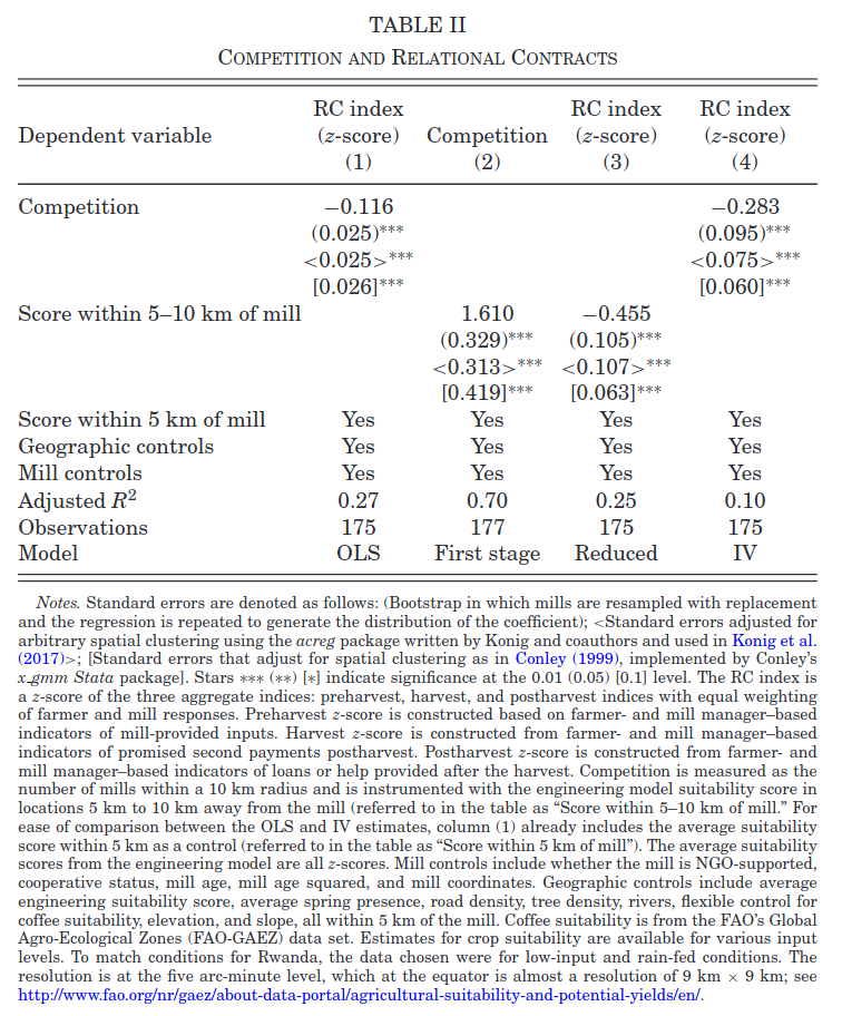
In “Competition and Relational Contracts in the Rwanda Coffee Chain,” Macchiavello and Morjaria (2020) examine how more competition can lead to worse outcomes in an environment without formal contracts. The authors create an index of “relational contracting” between farmers and mills. Relational contracting consists of loans, delayed payments, and so on that are sustained by repeated interaction instead of any formal contract enforcement. The authors then want to estimate how competition (the number of mills) affects relational contracting.
3.1 OLS
The authors estimate \[ RC_m = \alpha + \beta C_m + \eta X_m + \gamma Z_m + \epsilon_m \] where \(RC_m\) is a relational contracting index for mill \(m\), \(C_m\) is the number of competing mills within 10km of mill \(m\), \(X_m\) are mill characteristics, and \(Z_m\) are geographic characteristics of the land around the mill.
Give one reason why \(\Er[C_m \epsilon_m]\) might not be zero, speculate on the sign of \(\Er[C_m \epsilon_m]\), and say whether whether you expect \(\hat{\beta}^{OLS}\) to be greater or less than \(\beta\).
3.2 Instrument
As an instrument for \(C_m\), the authors use the predicted number of mills 5-10km away from an engineering model of coffee production. It predicts mill locations based on geography and local climate. Column (2) of Table II shows estimates of the first stage regression of \(C_m\) on this instrument. What assumption can we check by looking at this regression? Are you confident that this assumption is met? If not, what should be done about it? Hint:\(F=t^2 \approx \left(\frac{1.6}{0.4}\right)^2 \approx 16\).
3.3 Dependence
The sample consists of mills in Rwanda, some of which might be near one another. Briefly, how does this affect the consistency and asymptotic distribution of the estimates of \(\beta\) in Table II? What in the table, if anything, needs to be calculated differently than if observations were independent?
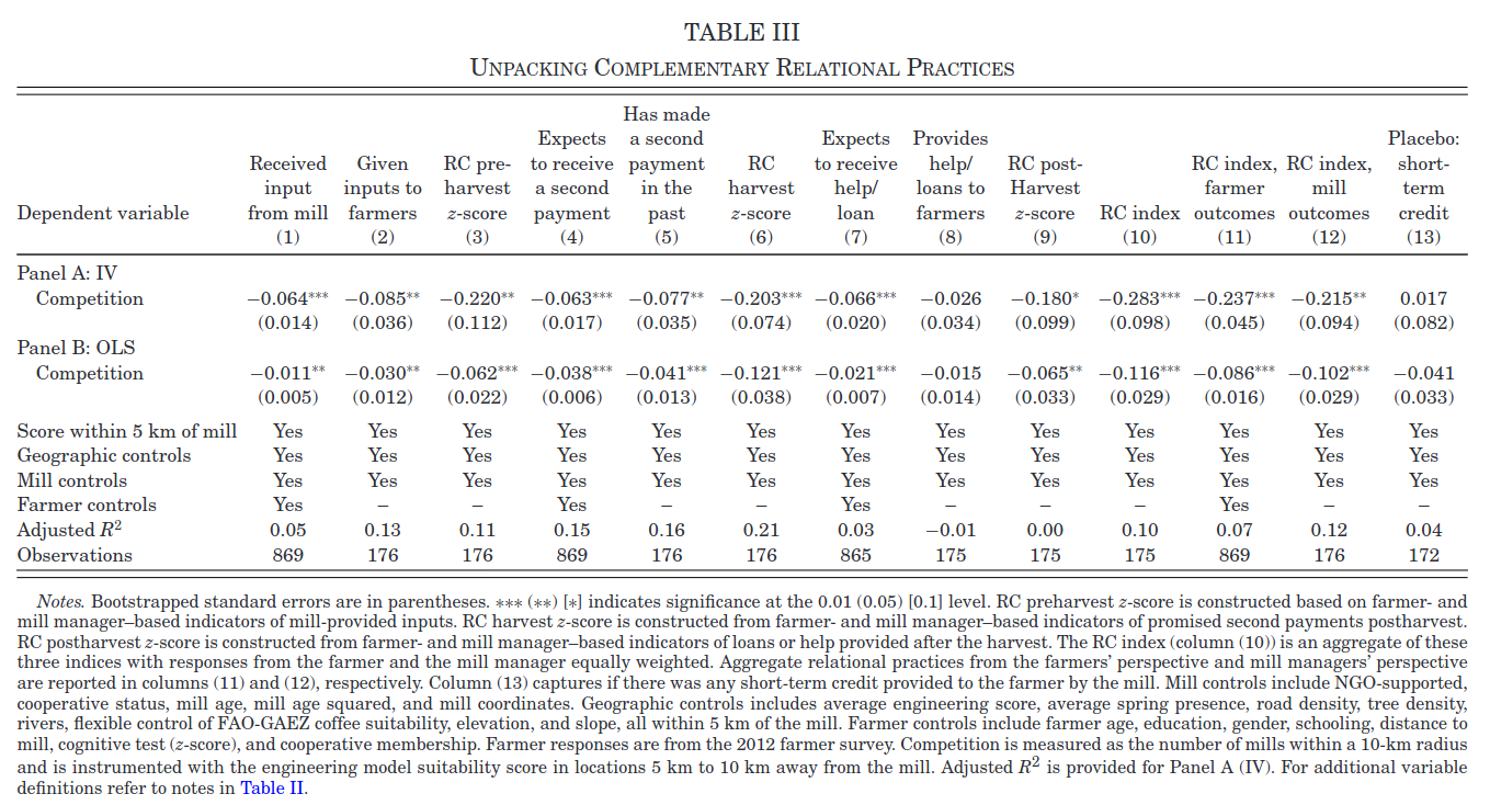
3.4 More Outcomes
Table 3 shows estimates of the same model as table 2, except instead of the relational contracting index as the outcome, the outcome is one of the components of the index. Different columns show different components. As shown, the coefficients are all negative and most are statistically significant. Should this make us less concerned about the potential weak instrument problem? Why or why not? Hint: these regressions all have the same first stage. A really good answer to this question would be fairly precise and perhaps derive the joint distribution of these estimates under weak instrument asymptotitcs.