Fixed Effects

ECON526

Paul Schrimpf

University of British Columbia

Table of contents

• Introduction
• Mechanics of Fixed Effects
• Some Theory

Introduction

Panel Data

• Units \(i=1,..., n\)
  • Ex: people, firms, cities, countries
• Time \(t=1,..., T\)
• Observe \(\left\{(y_{it}, X_{it})\right\}_{i=1,t=1}^{n,T}\)

Linear Model

• Model \[ y_{it} = X_{it}'\beta + \overbrace{U_i'\gamma + \epsilon_{it}}^{\text{unobserved}} \]

  • Time invariant confounders \(U_i\)

• Subtract individual averages \[ \begin{align*} y_{it} - \bar{y}_i & = (X_{it} - \bar{X}_i)'\beta + (\epsilon_{it} - \bar{\epsilon}_i) \\ \ddot{y}_{it} & = \ddot{X}_{it}' \beta + \ddot{\epsilon}_{it} \end{align*} \]

• Equivalent to estimating with individual dummies \[ y_{it} = X_{it}'\beta + \alpha_i + \epsilon_{it} \]

• Eliminates \(U_i\) and any time invariant observed \(X_i\)

Mechanics of Fixed Effects

\[ \def\Er{{\mathrm{E}}} \def\En{{\mathbb{E}_n}} \def\cov{{\mathrm{Cov}}} \def\var{{\mathrm{Var}}} \def\R{{\mathbb{R}}} \newcommand\norm[1]{\left\lVert#1\right\rVert} \def\rank{{\mathrm{rank}}} \newcommand{\inpr}{ \overset{p^*_{\scriptscriptstyle n}}{\longrightarrow}} \def\inprob{{\,{\buildrel p \over \rightarrow}\,}} \def\indist{\,{\buildrel d \over \rightarrow}\,} \DeclareMathOperator*{\plim}{plim} \]

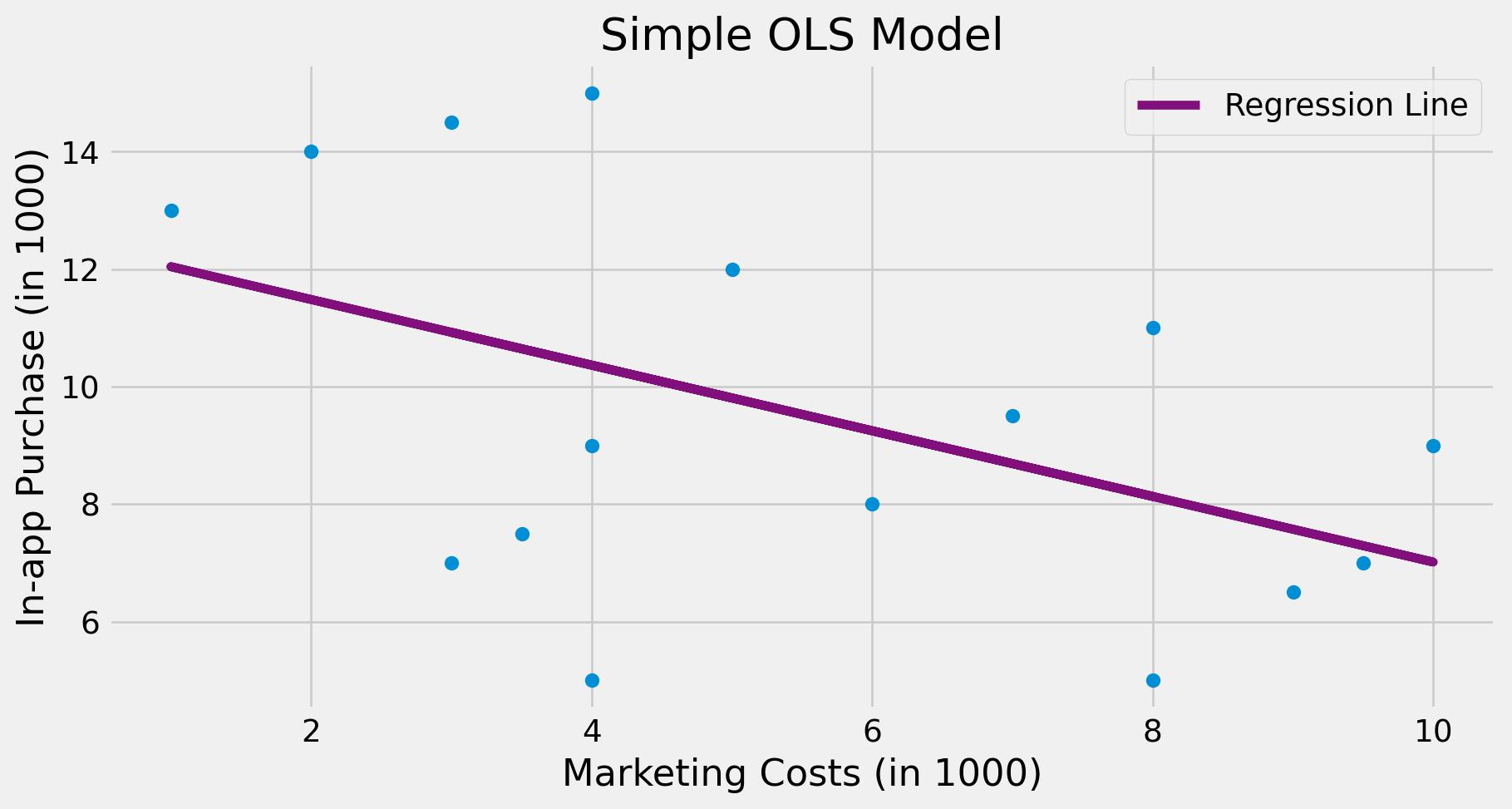
OLS

import warnings
warnings.filterwarnings('ignore')

import pandas as pd
import numpy as np
from matplotlib import style
from matplotlib import pyplot as plt
import statsmodels.formula.api as smf
style.use("fivethirtyeight")

¹

toy_panel = pd.DataFrame({
    "mkt_costs":[5,4,3.5,3, 10,9.5,9,8, 4,3,2,1, 8,7,6,4],
    "purchase":[12,9,7.5,7, 9,7,6.5,5, 15,14.5,14,13, 11,9.5,8,5],
    "city":["C0","C0","C0","C0", "C2","C2","C2","C2", "C1","C1","C1","C1", "C3","C3","C3","C3"]
})

m = smf.ols("purchase ~ mkt_costs", data=toy_panel).fit()

plt.scatter(toy_panel.mkt_costs, toy_panel.purchase)
plt.plot(toy_panel.mkt_costs, m.fittedvalues, c="C5", label="Regression Line")
plt.xlabel("Marketing Costs (in 1000)")
plt.ylabel("In-app Purchase (in 1000)")
plt.title("Simple OLS Model")
plt.legend();

1. Code from Facure (2022)

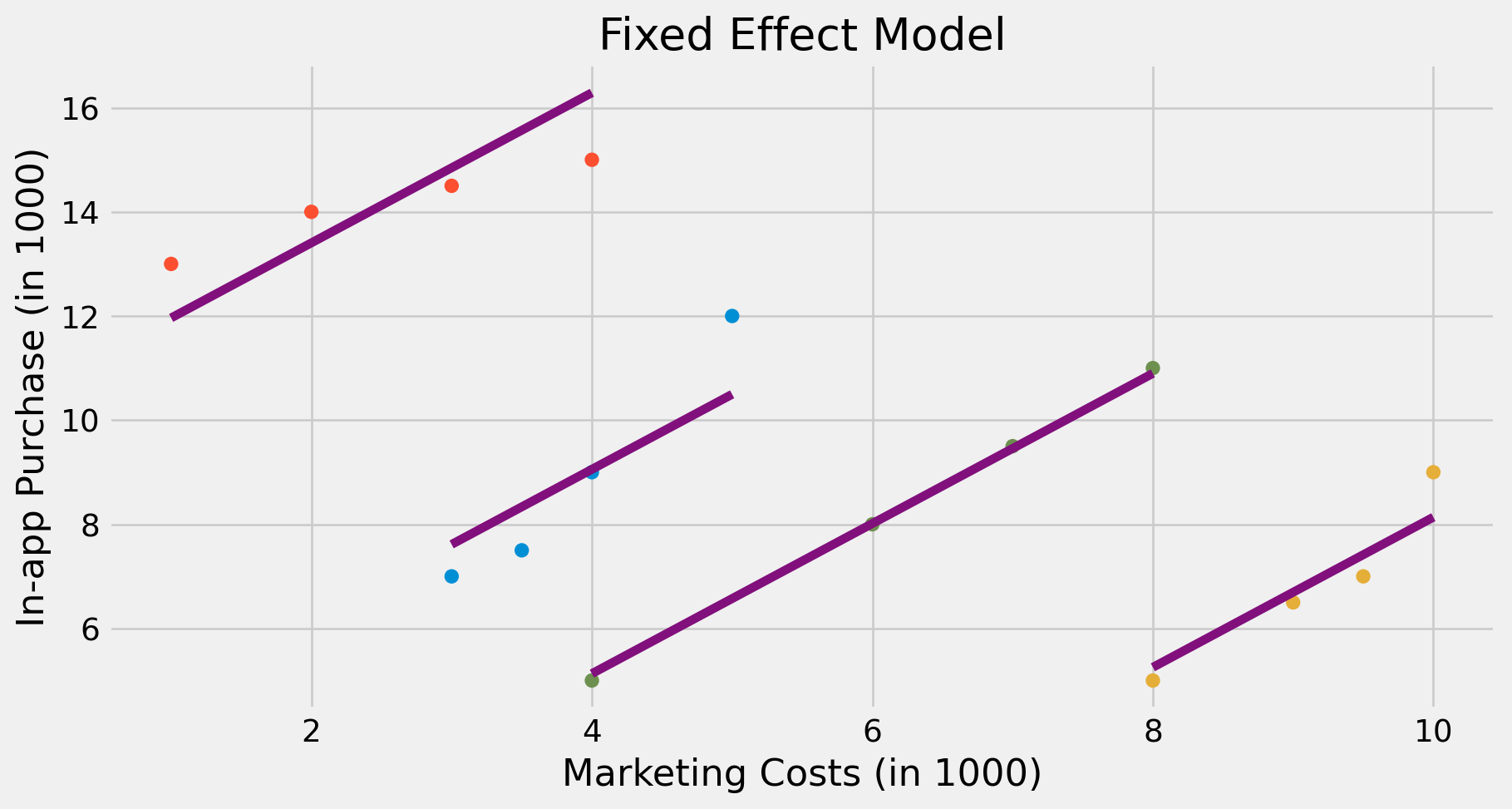
Fixed Effects / Within

¹

fe = smf.ols("purchase ~ mkt_costs + C(city)", data=toy_panel).fit()

fe_toy = toy_panel.assign(y_hat = fe.fittedvalues)

plt.scatter(toy_panel.mkt_costs, toy_panel.purchase, c=toy_panel.city)
for city in fe_toy["city"].unique():
    plot_df = fe_toy.query(f"city=='{city}'")
    plt.plot(plot_df.mkt_costs, plot_df.y_hat, c="C5")

plt.title("Fixed Effect Model")
plt.xlabel("Marketing Costs (in 1000)")
plt.ylabel("In-app Purchase (in 1000)");

1. Code from Facure (2022)

Some Theory

What Fixed Effects Cannot Fix

• Fixed effects corrects for time-invariant unobserved confounders, but

• Cannot fix:
  • Time-varying confounders
  • Reverse causality
  • Can make some biases worse if “between” \(i\) variation in \(X_{it}\) is useful (e.g. measurement error)

Strict Exogeneity

• In fixed effect model \[ y_{it} - \bar{y}_i = (X_{it} - \bar{X}_i)'\beta + (\epsilon_{it} - \bar{\epsilon}_i) \] for \(\hat{\beta}^{FE} \inprob \beta\), need \(\Er[(X_{it} - \bar{X}_i)(\epsilon_{it} - \bar{\epsilon}_i)]=0\)

• I.e. \(\Er[X_{it} \epsilon_{is}] = 0\) for all \(t, s\)

Strict Exogeneity

• Problematic with dynamics, e.g.
  • \(X_{it}\) including lagged \(y_{it-1}\)
  • \(X_{it}\) affected by past \(y\)
  • “Nickell bias”
• See Chen, Chernozhukov, and Fernández-Val (2019) for bias correction under weak exogeneity, \(\Er[X_{it} \epsilon_{is}] = 0\) for \(t \leq s\)

Standard Errors

• Generally, good idea to use clustered standard errors, clustered on \(i\)
• See MacKinnon, Nielsen, and Webb (2023) for guide to clustered standard errors

import pyfixest as pf
pf.feols('purchase ~ mkt_costs | city', data=toy_panel, vcov={'CRV1': 'city'}).summary()

###

Estimation:  OLS
Dep. var.: purchase, Fixed effects: city
Inference:  CRV1
Observations:  16

| Coefficient   |   Estimate |   Std. Error |   t value |   Pr(>|t|) |   2.5% |   97.5% |
|:--------------|-----------:|-------------:|----------:|-----------:|-------:|--------:|
| mkt_costs     |      1.441 |        0.307 |     4.700 |      0.018 |  0.465 |   2.417 |
---
RMSE: 0.689 R2: 0.954 R2 Within: 0.832 

Large \(n\), Small \(T\)

• Often \(n>>T\)
• Usual analysis of fixed effects uses asymptotics with \(n \to \infty\), \(T\) fixed
  • We will mostly stick to that, but if you have data with \(n \approx T\), other approaches can be better

Sources and Further Reading

• Facure (2022) chapter 14
• Huntington-Klein (2021) chapter 16

References

Chen, Shuowen, Victor Chernozhukov, and Iván Fernández-Val. 2019. “Mastering Panel Metrics: Causal Impact of Democracy on Growth.” AEA Papers and Proceedings 109 (May): 77–82. https://doi.org/10.1257/pandp.20191071.

Facure, Matheus. 2022. Causal Inference for the Brave and True. https://matheusfacure.github.io/python-causality-handbook/landing-page.html.

Huntington-Klein, Nick. 2021. The Effect: An Introduction to Research Design and Causality. CRC Press. https://theeffectbook.net/.

MacKinnon, James G., Morten Ørregaard Nielsen, and Matthew D. Webb. 2023. “Cluster-Robust Inference: A Guide to Empirical Practice.” Journal of Econometrics 232 (2): 272–99. https://doi.org/https://doi.org/10.1016/j.jeconom.2022.04.001.