Neural Networks

ECON526

Paul Schrimpf

University of British Columbia

Table of contents

• Introduction
• Double Descent and Overparameterization
• Software
• Uses for Neural Networks

Introduction

\[ \def\indep{\perp\!\!\!\perp} \def\Er{\mathrm{E}} \def\R{\mathbb{R}} \def\En{{\mathbb{E}_n}} \def\Pr{\mathrm{P}} \newcommand{\norm}[1]{\left\Vert {#1} \right\Vert} \newcommand{\abs}[1]{\left\vert {#1} \right\vert} \def\inprob{{\,{\buildrel p \over \rightarrow}\,}} \def\indist{\,{\buildrel d \over \rightarrow}\,} \DeclareMathOperator*{\plim}{plim} \DeclareMathOperator*{\argmax}{arg\,max} \DeclareMathOperator*{\argmin}{arg\,min} \]

Neural Networks

• Flexible function approximation & regression
• Automated feature engineering
• Exceptional performance on high dimensional data with low noise
  • Text
  • Images
  • Audio
  • Video

Single Layer Perceptron

• \(x_i \in \R^d\), want to approximate some \(f: \R^d \to \R\)
• Approximate by \[ \begin{align*} f(x_i; \mathbf{w},\mathbf{b}) = \psi_1 \left( \sum_{u=1}^m w_{u,1} \psi_0( x_i'w_{u,0} + b_{u,0}) + b_{u,1} \right) \end{align*} \] where
  • Weights: \(w_{u,1} \in \R\), \(w_{u,0} \in \R^d\)
  • Biases: \(b_{u,1}, b_{u,0} \in \R\)
  • Activation functions \(\psi_1, \psi_0: \R \to \R\)
  • Width: \(m\)

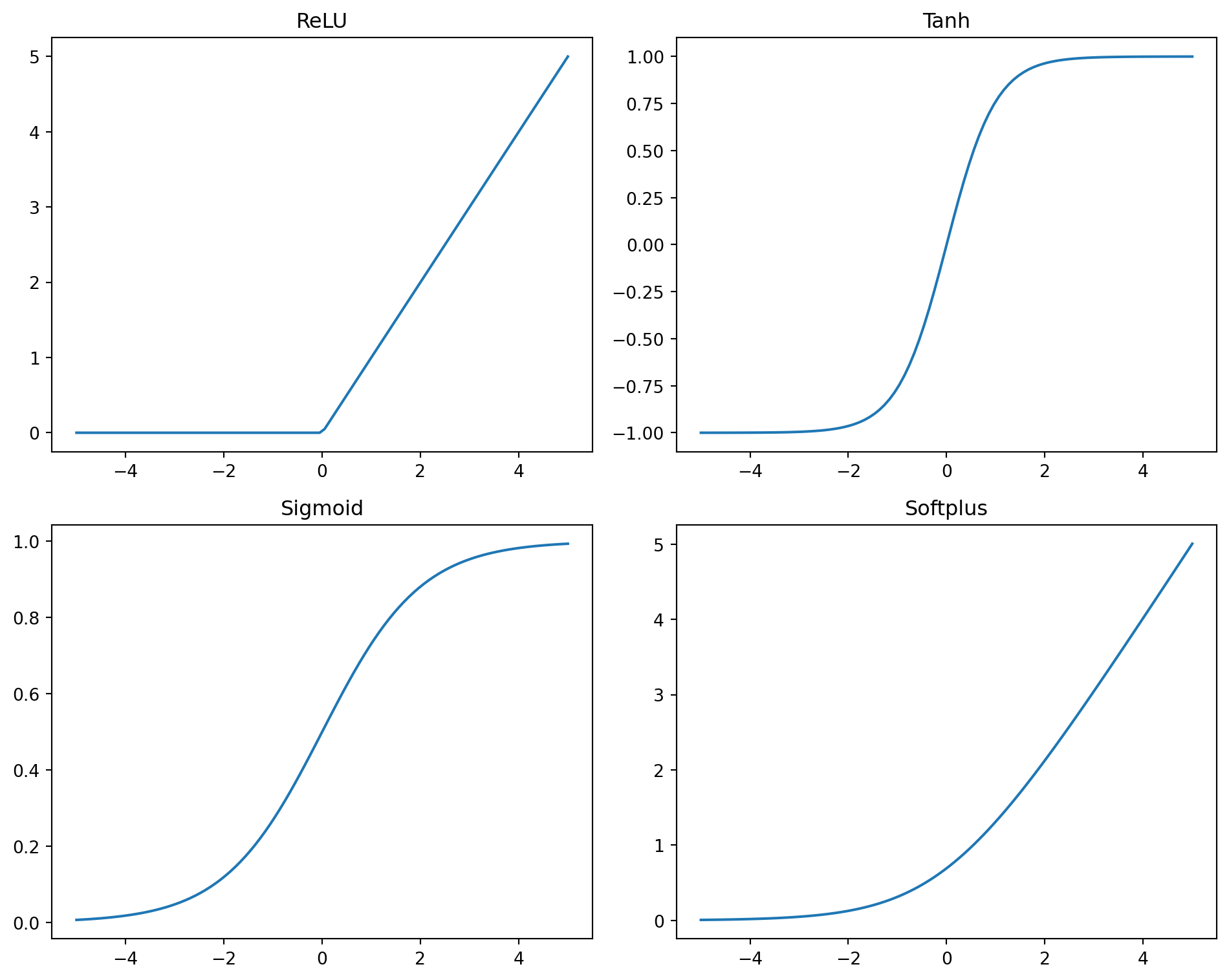
Activation functions

import numpy as np
import matplotlib.pyplot as plt
import torch.nn as nn
import torch
# plot 4 activation functions
x = torch.linspace(-5, 5, 100)
fig, ax = plt.subplots(2, 2, figsize=(10, 8))
ax = ax.flatten()
ax[0].plot(x, nn.ReLU()(x))
ax[0].set_title("ReLU")
ax[1].plot(x, nn.Tanh()(x))
ax[1].set_title("Tanh")
ax[2].plot(x, nn.Sigmoid()(x))
ax[2].set_title("Sigmoid")
ax[3].plot(x, nn.Softplus()(x))
ax[3].set_title("Softplus")
fig.tight_layout()
fig.show()

Single Layer Perceptron

import torch.nn as nn
import torch
class SingleLayerPerceptron(nn.Module):
    def __init__(self, d, m, activation=nn.ReLU()):
        super().__init__()
        self.d = d
        self.m = m
        self.activation = activation
        self.w0 = nn.Parameter(torch.randn(d, m))
        self.b0 = nn.Parameter(torch.randn(m))
        self.w1 = nn.Parameter(torch.randn(m))
        self.b1 = nn.Parameter(torch.randn(1))

    def forward(self, x):
        return self.activation(x @ self.w0 + self.b0) @ self.w1 + self.b1

Regression

• Data \(\{y_i, x_i\}_{i=1}^n\), \(x_i \in \R^d\), \(y_i \in \R\)
• Least squares: \[ \hat{\mathbf{w}}, \hat{\mathbf{b}} \in \argmin_{\mathbf{w},\mathbf{b}} \underbrace{\frac{1}{n} \sum_{i=1}^n \left(y_i - f(x_i; \mathbf{w},\mathbf{b}) \right)^2}_{\text{loss function}} \]
• Hard to find global minimum:
  • Loss not convex
  • Parameters very high dimensional

Gradient Descent

• Find approximate minimum instead \[ \overbrace{\hat{\theta}}^{\hat{\mathbf{w}}, \hat{\mathbf{b}}} \approx \argmin_{\theta} \ell(y, f(x;\theta)) \]
• Start with random \(\theta_1\)
• Repeatedly update: \[ \theta_{i+1} = \theta_i - \gamma \underbrace{\nabla \ell(y,f(;\theta))}_{\text{gradient}} \]
• Continue until loss stops improving
  • Optionally modify \(\gamma\) based on progress

Computing Gradients

• Automatic differentiation: automatically use chainrule on each step of computation
• E.g. \(\ell(\theta) = f(g(h(\theta)))\)
  • \(\ell : \R^p \to \R\), \(h: \R^p \to \R^q\), \(g: \R^q \to \R^j\), \(f: \R^j \to \R\) \[ \left(\nabla \ell(\theta)\riight)^T = \underbrace{Df_{g(h(\theta))}}_{1 \times j} \underbrace{Dg_{h(\theta)}}_{j \times q} \underbrace{Dh_\theta}_{q \times p} \]
• Forward mode:
  1. Calculate \(h(\theta)\) and \(D_1=Dh_\theta\)
  2. Calculate \(g(h(\theta))\) and \(Dg_{h(\theta)}\), multiply \(D_2=Dg_{h(\theta)} D_1\) (\(jqp\) scalar products and additions)
  3. Calculate \(f(g(h(\theta)))\) and \(Df_{g(h(\theta))}\), multiply \(Df_{g(h(\theta))} D_2\) (\(1jp\) scalar products and additions)
  • Work to propagate derivative \(\propto jqp + 1jp\)

Computing Gradients

• Reverse mode:
  1. “Forward pass” calculate and save \(h(\theta)\), \(g(h(\theta))\) and \(f(g(h(\theta)))\)
  2. “Back propagation”:
     1. Calculate \(D^r_1 = Df_{g(h(\theta))}\)
     2. Calculate \(D^r_2 = D^r_1 Dg_{h(\theta)}\) (\(1jq\) scalar products and additions)
     3. Calculate \(D^r_3 Dh_{\theta}\) (\(1qp\) scalar products and additions)
  • Work to propagate derivative \(\propto 1jq + 1qp\)
• Reverse mode much less work when \(p\) large

Gradient Descent

n = 100
sigma = 0.1
torch.manual_seed(987)
x = torch.randn(n,1)
f = np.vectorize(lambda x:  np.sin(x)+np.exp(-x*x)/(1+np.abs(x)))
y = torch.tensor(f(x), dtype=torch.float32) + sigma*torch.randn(x.shape)
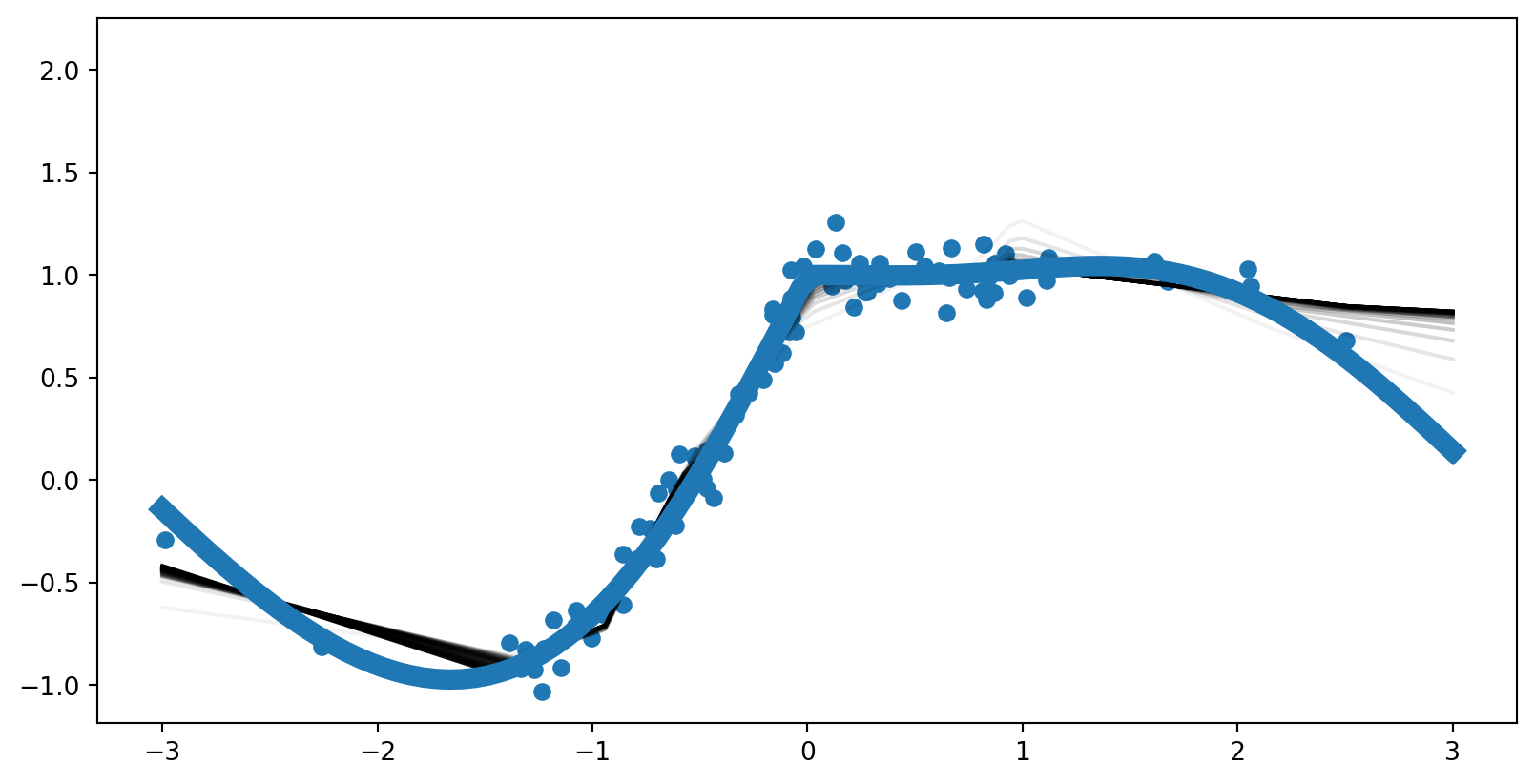
slp = SingleLayerPerceptron(1, 20, nn.ReLU())
lossfn = nn.MSELoss()
xlin = torch.linspace(-3,3,100)
fig, ax = plt.subplots()
epochs = 1000
stepscale = 0.1
for i in range(epochs):
    if (i % 50) == 0 :
        ax.plot(xlin,slp(xlin.reshape(-1,1)).data, alpha=i/epochs, color='k')
        slp.zero_grad()
    loss = lossfn(y.flatten(),slp(x))
    #print(f"{i}: {loss.item()}")
    # calculate gradient
    loss.backward()
    # access gradient & use to descend
    for p in slp.parameters():
        if p.requires_grad:
            p.data = p.data - stepscale*p.grad.data
            p.grad.data.zero_()
    slp.zero_grad()

ax.plot(xlin, f(xlin), label="f", lw=8)
ax.scatter(x.flatten(),y.flatten())
fig.show()

Multi Layer Perceptron

def multilayer(d,width,depth,activation=nn.ReLU()):
    mlp = nn.Sequential(
        nn.Linear(d,width),
        activation
    )
    for i in range(depth-1):
        mlp.add_module(f"layer {i+1}",nn.Linear(width, width))
        mlp.add_module(f"activation {i+1}",activation)


    mlp.add_module("output",nn.Linear(width,1))
    return(mlp)

mlp=multilayer(2, 10, 1, nn.ReLU())

def count_parameters(model):
    return sum(p.numel() for p in model.parameters() if p.requires_grad)

Multi Layer Perceptron

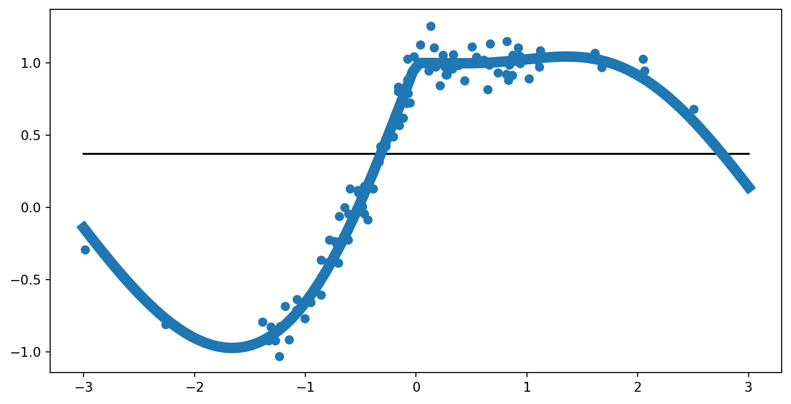
mlp = multilayer(1,4,4,nn.ReLU())
print(count_parameters(mlp))
optimizer = torch.optim.Adam(mlp.parameters(), lr=0.01)
fig, ax = plt.subplots()
epochs = 1000
for i in range(epochs):
    if (i % 50) == 0 :
        ax.plot(xlin,mlp(xlin.reshape(-1,1)).data, alpha=i/epochs, color='k')
        mlp.zero_grad()
    loss = lossfn(y,mlp(x))
    #print(f"{i}: {loss.item()}")
    optimizer.zero_grad()
    loss.backward()
    optimizer.step()

ax.plot(xlin, f(xlin), label="f", lw=8)
ax.scatter(x.flatten(),y.flatten())
fig.show()

73

Double Descent and Overparameterization

Overparameterization

• Classic statistics wisdom about nonparametric regression: as parameters increase:
  • Bias decreases
  • Variance increases
  • Need parameters \(<\) sample size for good performance
• Neural networks: often see best performance when parameters \(>\) sample size

Double Descent

from joblib import Parallel, delayed
#device = 'cuda' if torch.cuda.is_available() else 'cpu'
device = 'cpu' # problem is small, so not much help from cuda
num_epochs = 50
sims = 100
maxw = 10

def doubledescentdemo(x, y, xtest, ytest, f, device=device,
                      num_epochs=num_epochs, sims=sims,
                      maxw=maxw, lr=0.1):
    x=x.to(device)
    y=y.to(device).reshape(x.shape[0],1)
    fx = f(x.T).reshape(y.shape).to(device)
    ytest = ytest.to(device).reshape(xtest.shape[0],1)
    xtest = xtest.to(device)
    loss_fn = nn.MSELoss().to(device)

    losses = np.zeros([maxw,num_epochs,sims])
    nonoise = np.zeros([maxw,num_epochs,sims])

    def dd(w):
        mlp = multilayer(x.shape[1],w+1,1,nn.ReLU()).to(device)
        optimizer = torch.optim.Adam(mlp.parameters(), lr=lr)
        losses = np.zeros(num_epochs)
        nonoise=np.zeros(num_epochs)
        for n in range(num_epochs):
            y_pred = mlp(x)
            loss = loss_fn(y_pred, y)
            optimizer.zero_grad()
            loss.backward()
            optimizer.step()
            losses[n] = loss_fn(mlp(xtest),ytest).item()
            nonoise[n] = loss_fn(y_pred, fx)
            mlp.zero_grad()
        return([losses, nonoise])

    for w in range(maxw):
        foo=lambda s: dd(w)
        print(f"width {w}")
        results = Parallel(n_jobs=20)(delayed(foo)(s) for s in range(sims))

        for s in range(sims):
            losses[w,:,s] = results[s][0]
            nonoise[w,:,s] = results[s][1]
    return([losses, nonoise])

Double Descent

f = lambda x: np.exp(x[0]-x[1])
n = 20
torch.manual_seed(1234)
dimx = 5
x = torch.rand(n,dimx)
xtest = torch.rand(n,dimx)
sigma = 1.5
y = f(x.T) + sigma*torch.randn(x.shape[0])
ytest = f(xtest.T) + sigma*torch.randn(xtest.shape[0])
lr = 0.01
dd = doubledescentdemo(x, y, xtest, ytest, f, lr)

width 0

width 1
width 2
width 3
width 4
width 5
width 6
width 7
width 8
width 9

Double Descent

def plotdd(losses, nonoise):
    fig, ax = plt.subplots(2,2)
    ax = ax.flatten()
    ax[0].imshow(losses, cmap='plasma')
    ax[0].set_title('Test Loss')
    ax[0].set_xlabel('epoch')
    ax[0].set_ylabel('width')
    ax[1].imshow(nonoise, cmap='plasma')
    ax[1].set_title('error in f')
    ax[1].set_xlabel('epoch')
    ax[1].set_ylabel('width')

    ws = [0,1, 2, 4, 8]  #10, 12, 19]
    for w in ws:
        ax[2].plot(range(losses.shape[1]),losses[w,:], label=f"width={w+1}")
        ax[3].plot(range(nonoise.shape[1]),nonoise[w,:], label=f"width={w+1}")

    ax[2].set_xlabel('epoch')
    ax[2].set_ylabel('test loss')
    ax[2].legend()
    ax[3].set_xlabel('epoch')
    ax[3].set_ylabel('error in f')
    ax[3].legend()

    fig.tight_layout()

    return(fig)

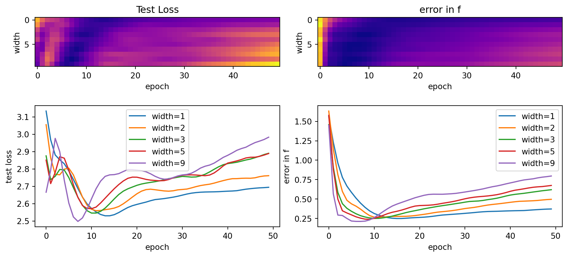
fig=plotdd(dd[0].mean(axis=2), dd[1].mean(axis=2))
fig.show()

Double Descent: Low Noise

sigma = 0.01
y = f(x.T) + sigma*torch.randn(x.shape[0])
ytest = f(xtest.T) + sigma*torch.randn(xtest.shape[0])
ddlowsig = doubledescentdemo(x,y,xtest,ytest,f, lr=0.05)

width 0
width 1
width 2
width 3
width 4
width 5
width 6
width 7
width 8
width 9

Double Descent: Low Noise

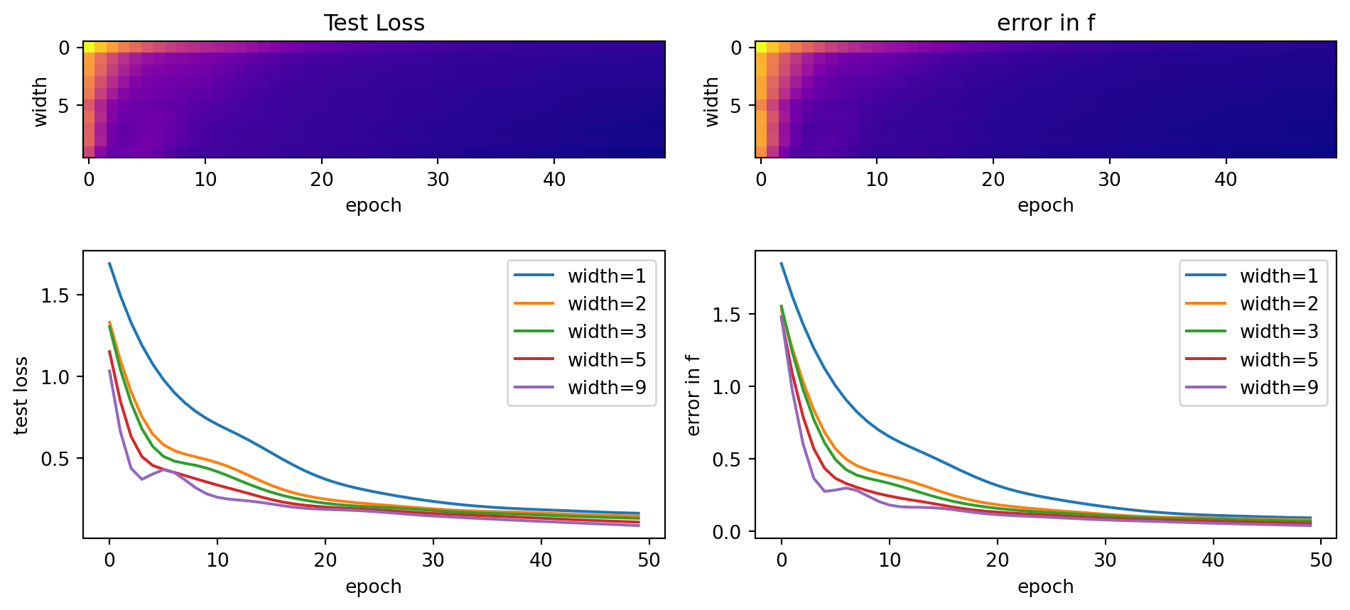
fig=plotdd(ddlowsig[0].mean(axis=2), ddlowsig[1].mean(axis=2))
fig.show()

Double Descent

• Figures show double descent in number of epochs, but has also been demonstrated with respect to number of parameters¹
• These simulations are quite fragile and depend on:
  • Form of \(f\)
  • dimension of \(x\)
  • noise in \(y\)
  • learning rate
  • optimizer

1. If you squint, you can sort of see double descent in parameters in these simulations too.

Software

Software

• PyTorch
  • Used above
  • Very popular
  • Middle ground between convenience and flexibility
  • Could be used via higher level wrapper (e.g. skorch)
• JAX
  • More extensible than pytorch
• Others: Tensorflow, Theano, Keras, and more

Uses for Neural Networks

Uses for Neural Networks

• Flexible regression and/or classification method, in double/debiased learning or elsewhere
  • Consider carefully whether difficulties of fitting are worth benefits
• Flexible function approximation
  • Useful for computing solutions to games, dynamic models, etc
• Text, images, audio
  • Use transfer learning

Transfer Learning

• Fit (or let researchers or company with more resources fit) large model on large, general dataset
• Find specialized data for your task
• Fine tune: take large model and update parameters with your data
• https://huggingface.co/ good source for large models to fine-tune

Other Architectures

• Multi-layer perceptrons / feed forward networks are the simplest neural networks, many extensions and variations exist
• Tricks to help with vanishing gradients and numeric stability:
  • Normalization
  • Residual connections
• Variations motivated by sequential data:
  • Recurrent
  • Transformers
• Variations motivated by images:
  • Convolutions
  • GAN
  • Diffusion¹

1. The motivating idea of diffusion models is different than neural networks, but neural networks are commonly used as one of the parts of diffusion models.

Sources and Further Reading

• QuantEcon Datascience: Regression - Neural Networks

• QuantEcon: Intro to Artificial Neural Nets

• pytorch notebooks from 323

References