Linear Regression with Real Data

ECON526

Paul Schrimpf

University of British Columbia

Table of contents

• Real-Data Examples
• Bad Controls, Mediators, and Colliders
• Treatment Probabilities and Effect Heterogeneity
• Stratified Regression and Standard Errors
• A Real Sign Reversal
• Data Appendix
• References

Real-Data Examples

AI Usage

These slides were entirely generated by Deepseek V4.1 Flash. The original prompt was:

I am not super satisfied with the examples from (facure?) in the regression slides. They are contrived examples from synthetic data. I would like to replace them with examples based on real data from economics papers. Ideally we want example(s) that capture (1) the idea of a bad control / mediator / collider (2) when P(D|X) and E[Y1-Y0|X] vary, omitting X biases the results (3) saturated regression reduces SE for an RCT, and (4) the sign reversal demonstrated on the caution slide. Search openicpsr and other repos of paper replication files for potential datasets to demonstrate these things. If possible, download the 4 most promising datasets and create slides using them in a separate qmd file.

I added instructions to get novel examples, not common ones (at first, it suggested the LaLonde data), and to cite sources and track whether the data is redistributable.

There are some mistakes in the slides. The text and focus is also a bit off. I leave them here to demonstrate how raw AI output is not always satisfactory.

Why Replace the Synthetic Examples?

• The synthetic examples in regression.qmd are clean, but they are not economics.
• This deck uses four published replication datasets to illustrate:
  1. bad controls, mediators, and colliders;
  2. omitted variables when treatment probabilities and treatment effects vary;
  3. why stratified/saturated regression can reduce standard errors in an RCT;
  4. a real-data sign reversal.
• The examples are deliberately chosen so that the data and the original paper can be traced and cited.

The Four Datasets

Dataset	Paper	Main use here
Afrobarometer + slave exports	Nunn and Wantchekon (2011b)	bad control / mediator
Oregon Health Insurance Experiment	Finkelstein et al. (2012)	treatment-probability and effect heterogeneity
Project STAR	Krueger (1999); Achilles et al. (2008)	stratified regression and SEs
German city associations	Satyanath et al. (2017a)	sign reversal

Data Sources and Redistribution

Dataset	Source	Redistribute in this repo?
Nunn–Wantchekon	AEA/openICPSR, doi:10.3886/E112479V1; public mirror used by the code	No. The raw .dta is not committed. The code downloads it from a public course mirror; the original replication package is the citation above.
OHIE	Harvard Dataverse, doi:10.7910/DVN/SJG1ED	Yes, for the small processed extract. Original is CC0 with additional terms: no commercial use, no re-identification, and cite the data.
Project STAR	Harvard Dataverse, doi:10.7910/DVN/SIWH9F	Yes. CC0; a processed extract is included.
Bowling for Fascism	Harvard Dataverse, doi:10.7910/DVN/EE6I7N	Yes. CC0; a processed extract is included.

The Nunn–Wantchekon raw file is not redistributed here. If the download fails, obtain Nunn_Wantchekon_AER_2011.dta from the AEA/openICPSR package or from the public IQSS mirror linked in the code below.

Bad Controls, Mediators, and Colliders

Nunn and Wantchekon (2011)

• Question: did the transatlantic and Indian Ocean slave trades leave a legacy of mistrust in Africa?
• Treatment: ln_export_area, log slave exports per historical ethnic-group area.
• Outcome: trust in the local government council.
• Candidate control: perceived performance/quality of the local council.

import os
import warnings
import numpy as np
import pandas as pd
import requests
import statsmodels.formula.api as smf
import matplotlib.pyplot as plt

warnings.filterwarnings("ignore")

nunn_path = "data/replication/Nunn_Wantchekon_AER_2011.dta"
nunn_url = ("https://raw.githubusercontent.com/iqss/prefresher/main/"
            "data/input/Nunn_Wantchekon_AER_2011.dta")
if not os.path.exists(nunn_path):
    r = requests.get(nunn_url)
    r.raise_for_status()
    with open(nunn_path, "wb") as f:
        f.write(r.content)

nunn = pd.read_stata(nunn_path)
for c in ["isocode", "occupation", "religion", "living_conditions", "education"]:
    nunn[c] = nunn[c].astype("category")

nunn_vars = [
    "trust_local_council", "ln_export_area", "age", "age2", "male", "urban_dum",
    "occupation", "religion", "living_conditions", "education",
    "district_ethnic_frac", "frac_ethnicity_in_district", "isocode", "district",
    "local_council_performance", "council_listen", "corrupt_local_council",
]
nunn_d = nunn.dropna(subset=nunn_vars).copy()

Nunn and Wantchekon (2011)

• What happens when we add local-council quality?
• If council quality is a mediator, the coefficient is no longer the total effect.
• If council quality is a collider, conditioning opens a non-causal path.

nunn_models = {
    "(1) bivariate": "trust_local_council ~ ln_export_area",
    "(2) + individual controls": (
        "trust_local_council ~ ln_export_area + age + age2 + male + urban_dum "
        "+ C(occupation) + C(religion) + C(living_conditions) + C(education)"
    ),
    "(3) + country FE": (
        "trust_local_council ~ ln_export_area + age + age2 + male + urban_dum "
        "+ C(occupation) + C(religion) + C(living_conditions) + C(education) "
        "+ C(isocode)"
    ),
    "(4) + council performance": (
        "trust_local_council ~ ln_export_area + age + age2 + male + urban_dum "
        "+ C(occupation) + C(religion) + C(living_conditions) + C(education) "
        "+ C(isocode) + local_council_performance"
    ),
    "(5) + all council quality": (
        "trust_local_council ~ ln_export_area + age + age2 + male + urban_dum "
        "+ C(occupation) + C(religion) + C(living_conditions) + C(education) "
        "+ C(isocode) + local_council_performance + council_listen "
        "+ corrupt_local_council"
    ),
}
nunn_rows = []
for name, form in nunn_models.items():
    m = smf.ols(form, data=nunn_d).fit(
        cov_type="cluster", cov_kwds={"groups": nunn_d["district"]}
    )
    nunn_rows.append({
        "Specification": name,
        "Coefficient on ln(exports)": m.params["ln_export_area"],
        "SE": m.bse["ln_export_area"],
        "N": int(m.nobs),
    })
nunn_table = pd.DataFrame(nunn_rows).set_index("Specification")
print(nunn_table.round(3).to_markdown())

| Specification             |   Coefficient on ln(exports) |    SE |     N |
|:--------------------------|-----------------------------:|------:|------:|
| (1) bivariate             |                       -0.152 | 0.018 | 15748 |
| (2) + individual controls |                       -0.131 | 0.016 | 15748 |
| (3) + country FE          |                       -0.113 | 0.018 | 15748 |
| (4) + council performance |                       -0.077 | 0.015 | 15748 |
| (5) + all council quality |                       -0.059 | 0.014 | 15748 |

Nunn and Wantchekon (2011): Interpretation

• The coefficient falls from about \(-0.15\) to \(-0.06\) once council quality is included.
• The total effect of the slave trade includes any effect operating through local institutions.
• Holding council quality fixed changes the estimand from a total effect to a direct effect, and it can also open a collider path if unobserved local public goods affect both council quality and trust.
• This is the real-data version of the “bad control” warning: more controls are not always better.

Treatment Probabilities and Effect Heterogeneity

Oregon Health Insurance Experiment

• Lottery-based Medicaid expansion in Oregon.
• Treatment: selected in the lottery.
• Outcome: any doctor visit in the in-person survey.
• Randomization was not i.i.d. across household sizes: lottery odds varied with the number of eligible household members.

ohie = pd.read_csv("data/replication/ohie_analysis.csv")
ohie = ohie.dropna(subset=["doc_any", "treatment", "numhh"]).copy()
ohie["numhh"] = ohie["numhh"].astype(int)

prob_table = (
    ohie.groupby("numhh")
    .agg(P_treated=("treatment", "mean"), N=("treatment", "size"))
    .reset_index()
)
print(prob_table.round(3).to_markdown(index=False))

ohie_effects = []
for h in sorted(ohie["numhh"].unique()):
    g = ohie[ohie["numhh"] == h]
    m = smf.ols("doc_any ~ treatment", data=g).fit(cov_type="HC1")
    ohie_effects.append({
        "Household size": h,
        "Effect on P(doctor visit)": m.params["treatment"],
        "SE": m.bse["treatment"],
        "N": int(m.nobs),
    })
print("\n" + pd.DataFrame(ohie_effects).round(3).to_markdown(index=False))

|   numhh |   P_treated |    N |
|--------:|------------:|-----:|
|       1 |       0.493 | 9235 |
|       2 |       0.613 | 2952 |
|       3 |       0.889 |   18 |

|   Household size |   Effect on P(doctor visit) |    SE |    N |
|-----------------:|----------------------------:|------:|-----:|
|                1 |                       0.035 | 0.01  | 9235 |
|                2 |                       0.039 | 0.018 | 2952 |
|                3 |                       0.125 | 0.396 |   18 |

Oregon Health Insurance Experiment

• Simple difference versus adjustment for household size:

ohie_models = {
    "Simple difference": "doc_any ~ treatment",
    "+ household size": "doc_any ~ treatment + C(numhh)",
    "+ household size interactions": "doc_any ~ treatment * C(numhh)",
}
ohie_rows = []
for name, form in ohie_models.items():
    m = smf.ols(form, data=ohie).fit(cov_type="HC1")
    ohie_rows.append({
        "Specification": name,
        "Effect": m.params["treatment"],
        "SE": m.bse["treatment"],
        "N": int(m.nobs),
    })
print(pd.DataFrame(ohie_rows).set_index("Specification").round(4).to_markdown())

| Specification                 |   Effect |     SE |     N |
|:------------------------------|---------:|-------:|------:|
| Simple difference             |   0.0301 | 0.0085 | 12205 |
| + household size              |   0.036  | 0.0086 | 12205 |
| + household size interactions |   0.035  | 0.0097 | 12205 |

Oregon Health Insurance Experiment: What Is the Lesson?

• \(P(D=1\mid X)\) varies with household size: about 0.49, 0.61, and 0.89 in the analysis sample for one-, two-, and three-person households.
• The treatment effect also varies: the largest effects are for the largest households.
• With heterogeneous effects and non-constant propensity scores, the simple difference in means is a weighted average that need not equal the ATE.
• Adjusting for the randomization stratum changes the estimate and its interpretation.
• Here numhh is a good control: it is pre-treatment and determines treatment probabilities. It is not a mediator.

Stratified Regression and Standard Errors

Project STAR

• Tennessee class-size experiment: students were randomized to small classes, regular classes, or regular classes with a teacher’s aide.
• Outcome: kindergarten reading score.
• Treatment: small class versus regular class (aide classes omitted for this comparison).
• School is a randomization stratum; baseline covariates are available.

star = pd.read_csv("data/replication/star_k.csv")
star = star[star["classtype"].isin([1, 2])].copy()
star["small"] = (star["classtype"] == 1).astype(int)
star = star.dropna(subset=["read", "small", "school", "gender", "race", "freelunch"])

star_models = {
    "Simple difference": "read ~ small",
    "+ school FE": "read ~ small + C(school)",
    "+ school FE + covariates": "read ~ small + C(school) + gender + race + freelunch",
}
star_rows = []
for name, form in star_models.items():
    m = smf.ols(form, data=star).fit(cov_type="HC1")
    star_rows.append({
        "Specification": name,
        "Effect of small class": m.params["small"],
        "SE": m.bse["small"],
        "N": int(m.nobs),
    })
print(pd.DataFrame(star_rows).set_index("Specification").round(3).to_markdown())

| Specification            |   Effect of small class |    SE |    N |
|:-------------------------|------------------------:|------:|-----:|
| Simple difference        |                   5.899 | 1.044 | 3733 |
| + school FE              |                   6.702 | 0.979 | 3733 |
| + school FE + covariates |                   6.722 | 0.943 | 3733 |

Project STAR: Interpretation

• The point estimate is stable at roughly 6–7 points.
• Controlling for the randomization stratum (school) and baseline covariates reduces the standard error by about 10 percent.
• That is the intuition behind saturated/stratified regression in an RCT: removing predictable between-stratum variation in outcomes sharpens the treatment contrast.
• With many strata, fully interacting treatment with every stratum can be noisy; additive stratum effects are often the practical compromise.

A Real Sign Reversal

Bowling for Fascism

• Satyanath et al. (2017a) study 229 German towns and cities in the 1920s.
• Treatment: association density (clubs per capita).
• Outcome: total Nazi Party entries by early 1933.
• A bivariate regression says denser association networks are associated with fewer Nazi entries. Is that credible?

bowling = pd.read_csv("data/replication/bowling_cities.csv")
bowling["high_clubs"] = (bowling["clubs_all_pc"] >
                         bowling["clubs_all_pc"].median()).astype(int)

bowling_models = {
    "Bivariate": "NSentry_total ~ clubs_all_pc",
    "+ log population": "NSentry_total ~ clubs_all_pc + lnpop",
    "+ population controls": (
        "NSentry_total ~ clubs_all_pc + lnpop + share_cath25 "
        "+ bcollar25 + share_jew25 + unemp33"
    ),
    "Binary density + controls": (
        "NSentry_total ~ high_clubs + lnpop + share_cath25 "
        "+ bcollar25 + share_jew25 + unemp33"
    ),
}
bowling_rows = []
for name, form in bowling_models.items():
    m = smf.ols(form, data=bowling).fit(cov_type="HC1")
    key = "clubs_all_pc" if "clubs_all_pc" in m.params else "high_clubs"
    bowling_rows.append({
        "Specification": name,
        "Effect": m.params[key],
        "SE": m.bse[key],
        "N": int(m.nobs),
    })
print(pd.DataFrame(bowling_rows).set_index("Specification").round(3).to_markdown())

| Specification             |   Effect |    SE |   N |
|:--------------------------|---------:|------:|----:|
| Bivariate                 |  -16.399 | 3.224 | 229 |
| + log population          |    6.967 | 2.513 | 229 |
| + population controls     |    6.088 | 2.486 | 227 |
| Binary density + controls |   15.628 | 5.938 | 227 |

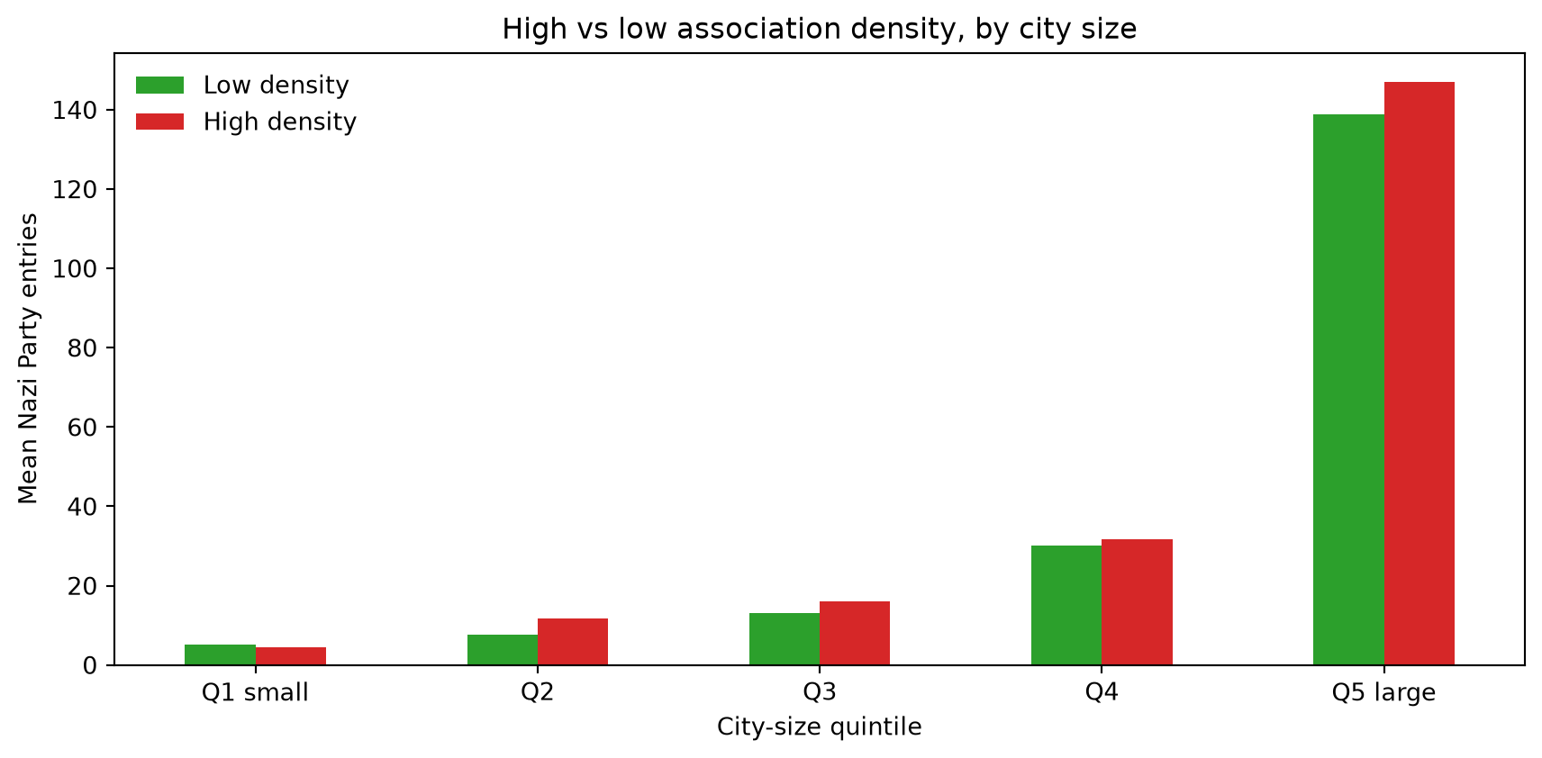
Bowling for Fascism: The Sign Reversal

bowling["pop_quintile"] = pd.qcut(
    bowling["lnpop"], 5, labels=["Q1 small", "Q2", "Q3", "Q4", "Q5 large"]
)
means = (
    bowling.groupby(["pop_quintile", "high_clubs"], observed=True)["NSentry_total"]
    .mean()
    .unstack()
)
print(means.round(1).to_markdown())

fig, ax = plt.subplots(figsize=(9, 4.5))
means.plot(kind="bar", ax=ax, color=["C2", "C3"])
ax.set_xlabel("City-size quintile")
ax.set_ylabel("Mean Nazi Party entries")
ax.set_title("High vs low association density, by city size")
ax.legend(["Low density", "High density"], frameon=False)
plt.xticks(rotation=0)
plt.tight_layout()
plt.show()

| pop_quintile   |     0 |     1 |
|:---------------|------:|------:|
| Q1 small       |   5.1 |   4.5 |
| Q2             |   7.6 |  11.6 |
| Q3             |  13.2 |  16.1 |
| Q4             |  30   |  31.6 |
| Q5 large       | 138.9 | 147   |

Bowling for Fascism: Interpretation

• The bivariate slope is negative: denser association networks look like they slowed Nazi entry.
• But association density is much higher in small towns, and small towns have far fewer total entries.
• Adding log population flips the coefficient from about \(-16.4\) to \(+7.0\); with controls it remains positive.
• In four of the five city-size quintiles, high-density towns have more Nazi entries; the bivariate result is driven by the smallest towns.
• This is a real-data version of the caution slide: a linear regression is a best linear approximation, not a guarantee that the sign answers the causal question.
• The paper’s own conclusion is that denser social networks were associated with faster Nazi Party entry.

Data Appendix

Reproducing the Extracts

sources = pd.DataFrame([
    {
        "Dataset": "Nunn--Wantchekon",
        "Local file": "data/replication/Nunn_Wantchekon_AER_2011.dta",
        "Original source": "https://doi.org/10.3886/E112479V1",
        "Redistributed": "No",
    },
    {
        "Dataset": "OHIE",
        "Local file": "data/replication/ohie_analysis.csv",
        "Original source": "https://doi.org/10.7910/DVN/SJG1ED",
        "Redistributed": "Yes (processed extract; CC0 + terms)",
    },
    {
        "Dataset": "Project STAR",
        "Local file": "data/replication/star_k.csv",
        "Original source": "https://doi.org/10.7910/DVN/SIWH9F",
        "Redistributed": "Yes (processed extract; CC0)",
    },
    {
        "Dataset": "Bowling for Fascism",
        "Local file": "data/replication/bowling_cities.csv",
        "Original source": "https://doi.org/10.7910/DVN/EE6I7N",
        "Redistributed": "Yes (processed extract; CC0)",
    },
])
print(sources.to_markdown(index=False))

| Dataset             | Local file                                    | Original source                    | Redistributed                        |
|:--------------------|:----------------------------------------------|:-----------------------------------|:-------------------------------------|
| Nunn--Wantchekon    | data/replication/Nunn_Wantchekon_AER_2011.dta | https://doi.org/10.3886/E112479V1  | No                                   |
| OHIE                | data/replication/ohie_analysis.csv            | https://doi.org/10.7910/DVN/SJG1ED | Yes (processed extract; CC0 + terms) |
| Project STAR        | data/replication/star_k.csv                   | https://doi.org/10.7910/DVN/SIWH9F | Yes (processed extract; CC0)         |
| Bowling for Fascism | data/replication/bowling_cities.csv           | https://doi.org/10.7910/DVN/EE6I7N | Yes (processed extract; CC0)         |

Data Notes

• Nunn–Wantchekon: the raw file is not redistributed. The code downloads the public IQSS mirror; the authoritative replication package is Nunn and Wantchekon (2011a) at openICPSR. If you need to download it manually, use the DOI and place the file at data/replication/Nunn_Wantchekon_AER_2011.dta.
• OHIE: the processed extract keeps only analysis variables and drops direct identifiers. The original is CC0 with additional terms: no commercial use, no re-identification, and citation of Finkelstein and Baicker (2012). See the Dataverse record for the full terms.
• Project STAR: CC0. The processed extract is star_k.csv; the original deposit is Achilles et al. (2008).
• Bowling for Fascism: CC0. The processed extract is bowling_cities.csv; the original deposit is Satyanath et al. (2017b).

Source Citations

• Nunn and Wantchekon (2011b); replication package: Nunn and Wantchekon (2011a).
• Finkelstein et al. (2012); data: Finkelstein and Baicker (2012).
• Krueger (1999); data: Achilles et al. (2008).
• Satyanath et al. (2017a); data: Satyanath et al. (2017b).

References

Achilles, C. M., H. P. Bain, F. Bellott, et al. 2008. Tennessee’s Student Teacher Achievement Ratio (STAR) Project. Harvard Dataverse. https://doi.org/10.7910/DVN/SIWH9F.

Finkelstein, Amy, and Katherine Baicker. 2012. Oregon Health Insurance Experiment: Public Use Data. Harvard Dataverse. https://doi.org/10.7910/DVN/SJG1ED.

Finkelstein, Amy, Sarah Taubman, Bill Wright, et al. 2012. “The Oregon Health Insurance Experiment: Evidence from the First Year.” Quarterly Journal of Economics 127 (3): 1057–106. https://doi.org/10.1093/qje/qjs020.

Krueger, Alan B. 1999. “Experimental Estimates of Education Production Functions.” Quarterly Journal of Economics 114 (2): 497–532. https://doi.org/10.1162/003355399556052.

Nunn, Nathan, and Leonard Wantchekon. 2011a. Replication Data for: The Slave Trade and the Origins of Mistrust in Africa. AEA Data and Code Repository, openICPSR. https://doi.org/10.3886/E112479V1.

Nunn, Nathan, and Leonard Wantchekon. 2011b. “The Slave Trade and the Origins of Mistrust in Africa.” American Economic Review 101 (7): 3221–52. https://doi.org/10.1257/aer.101.7.3221.

Satyanath, Shanker, Nico Voigtländer, and Hans-Joachim Voth. 2017a. “Bowling for Fascism: Social Capital and the Rise of the Nazi Party.” Journal of Political Economy 125 (2): 478–526. https://doi.org/10.1086/690949.

Satyanath, Shanker, Nico Voigtländer, and Hans-Joachim Voth. 2017b. Code and Data for: Bowling for Fascism: Social Capital and the Rise of the Nazi Party. Harvard Dataverse. https://doi.org/10.7910/DVN/EE6I7N.