Synthetic Control
ECON526
Cigarette Sales Trends
ax = plt.subplot(1, 1, 1)
for gdf in cigar.groupby("state"):
    ax.plot(gdf[1]['year'],gdf[1]['cigsale'], alpha=0.2, lw=1, color="k")

ax.set_ylim(40, 150)
ax.plot(cigar.query("california")['year'], cigar.query("california")['cigsale'], label="California")
cigar.query("not california").groupby("year")['cigsale'].mean().plot(ax=ax, label="Mean Other States")

plt.vlines(x=1988, ymin=40, ymax=140, linestyle=":", lw=2, label="Proposition 99")
plt.ylabel("Per-capita cigarette sales (in packs)")
plt.legend()
plt.show()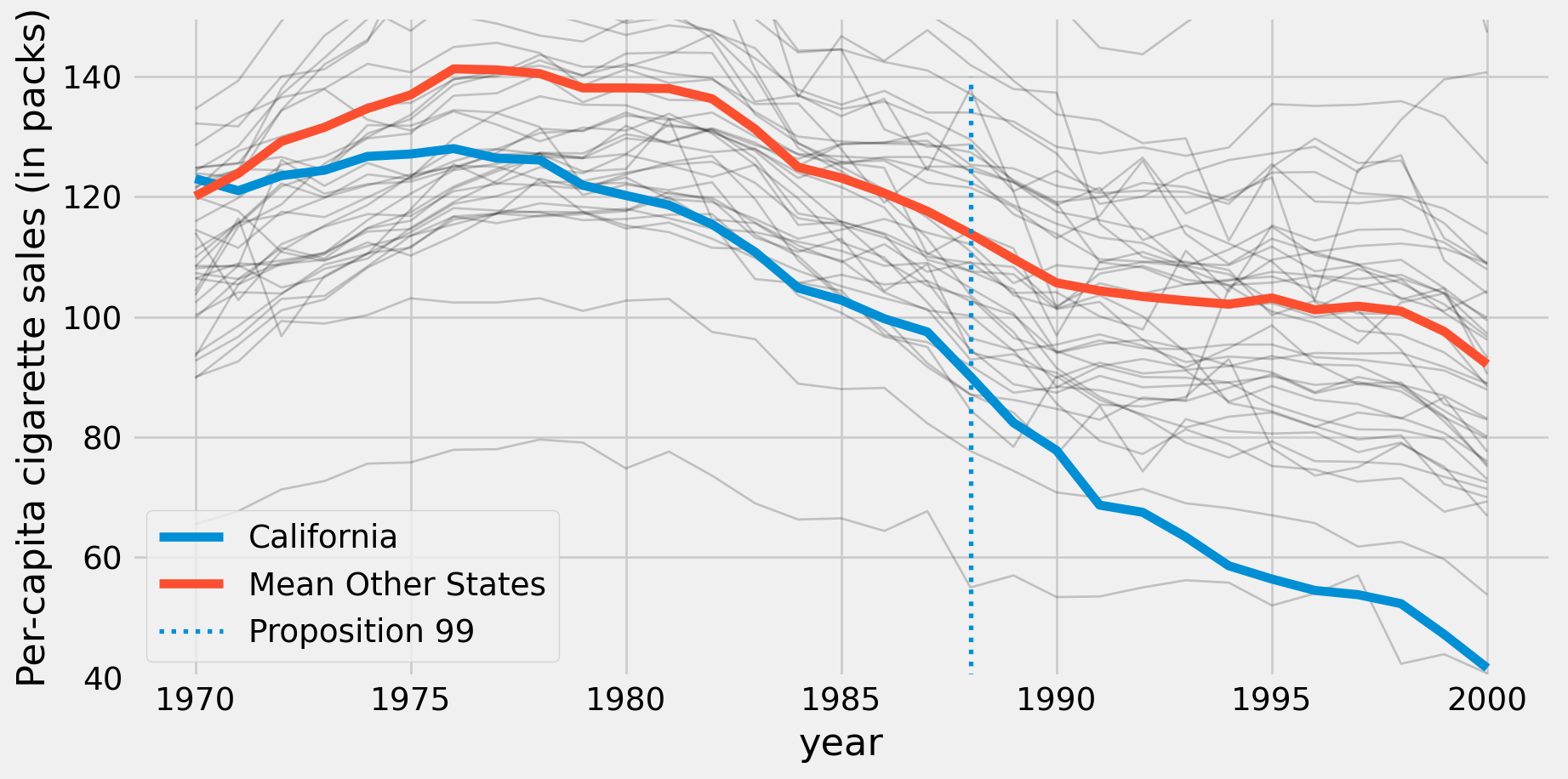
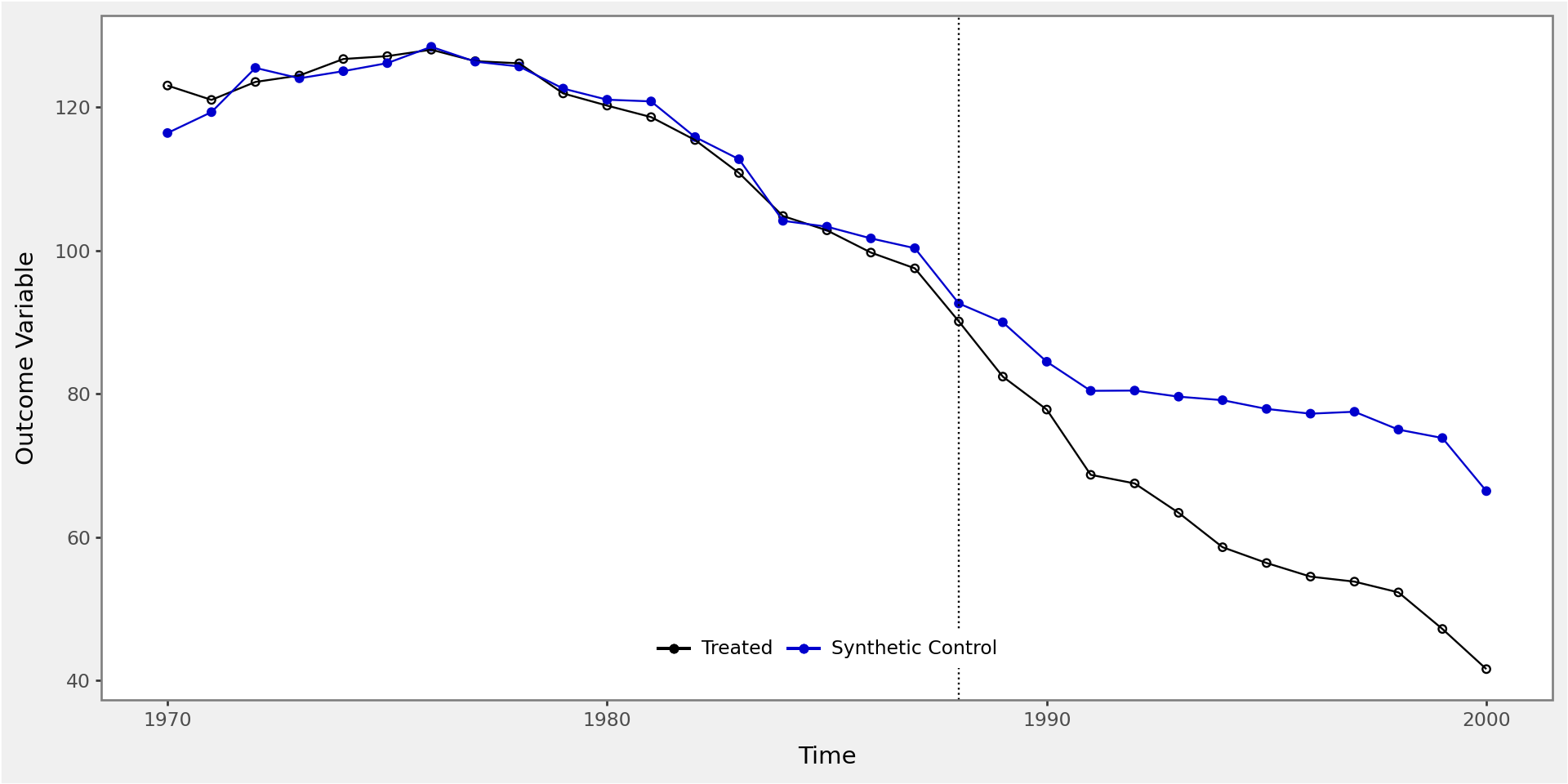
Effect of California Tobacco Control Program
calif_synth = cigar.query("~california").pivot(index='year', columns="state")["cigsale"].values.dot(calif_weights)
plt.figure(figsize=(10,6))
plt.plot(cigar.query("california")["year"], cigar.query("california")["cigsale"], label="California")
plt.plot(cigar.query("california")["year"], calif_synth, label="Synthetic Control")
plt.vlines(x=1988, ymin=40, ymax=140, linestyle=":", lw=2, label="Proposition 99")
plt.ylabel("Per-capita cigarette sales (in packs)")
plt.legend()
plt.show()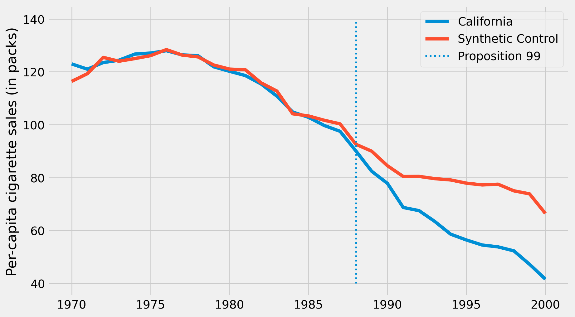
Treatment Permutation
Code
plt.figure(figsize=(12,7))
for state in synthetic_states:
    plt.plot(state["year"], state["cigsale"] - state["synthetic"], color="C5",alpha=0.4)

plt.plot(cigar.query("california")["year"], cigar.query("california")["cigsale"] - calif_synth,
        label="California");

plt.vlines(x=1988, ymin=-50, ymax=120, linestyle=":", lw=2, label="Proposition 99")
plt.hlines(y=0, xmin=1970, xmax=2000, lw=3)
plt.ylabel("Gap in per-capita cigarette sales (in packs)")
plt.title("State - Synthetic Across Time")
plt.legend()
plt.show()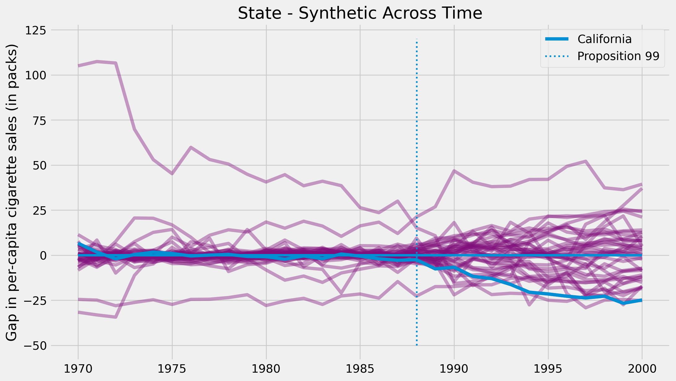
Treatment Permutation Inference
Code
def pre_treatment_error(state):
    pre_treat_error = (state.query("~after_treatment")["cigsale"]
                       - state.query("~after_treatment")["synthetic"]) ** 2
    return pre_treat_error.mean()

plt.figure(figsize=(12,7))
for state in synthetic_states:

    # remove units with mean error above 80.
    if pre_treatment_error(state) < 80:
        plt.plot(state["year"], state["cigsale"] - state["synthetic"], color="C5",alpha=0.4)

plt.plot(cigar.query("california")["year"], cigar.query("california")["cigsale"] - calif_synth,
        label="California");

plt.vlines(x=1988, ymin=-50, ymax=120, linestyle=":", lw=2, label="Proposition 99")
plt.hlines(y=0, xmin=1970, xmax=2000, lw=3)
plt.ylabel("Gap in per-capita cigarette sales (in packs)")
plt.title("Distribution of Effects")
plt.title("State - Synthetic Across Time (Large Pre-Treatment Errors Removed)")
plt.legend()
plt.show()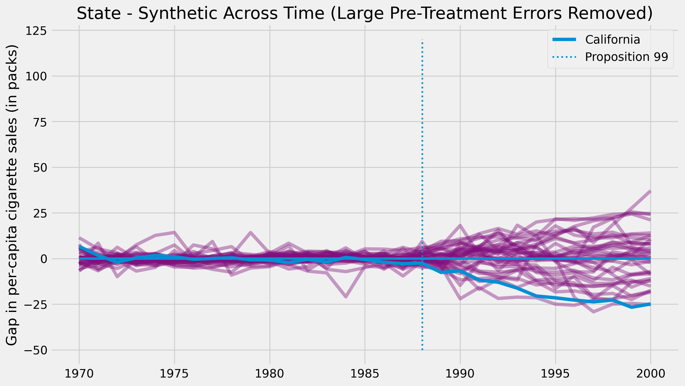
Point Estimation
Code
-----------------------------------------------------------------------
Call: scest
Synthetic Control Estimation - Setup

Constraint Type:                                                simplex
Constraint Size (Q):                                                  1
Treated Unit:                                                         3
Size of the donor pool:                                              38
Features                                                              2
Pre-treatment period                                          1970-1988
Pre-treatment periods used in estimation per feature:
 Feature  Observations
 cigsale            19
retprice            19
Covariates used for adjustment per feature:
 Feature  Num of Covariates
 cigsale                  0
retprice                  0

Synthetic Control Estimation - Results

Active donors: 5

Coefficients:
                    Weights
Treated Unit Donor
3            1        0.000
             10       0.000
             11       0.000
             12       0.000
             13       0.000
             14       0.000
             15       0.000
             16       0.000
             17       0.000
             18       0.000
             19       0.000
             2        0.000
             20       0.000
             21       0.113
             22       0.105
             23       0.457
             24       0.000
             25       0.000
             26       0.000
             27       0.000
             28       0.000
             29       0.000
             30       0.000
             31       0.000
             32       0.000
             33       0.000
             34       0.240
             35       0.000
             36       0.000
             37       0.000
             38       0.000
             39       0.000
             4        0.000
             5        0.085
             6        0.000
             7        0.000
             8        0.000
             9        0.000

-----------------------------------------------------------------------
Call: scest
Synthetic Control Estimation - Setup

Constraint Type:                                          user provided
Constraint Size (Q):                                                  1
Treated Unit:                                                         3
Size of the donor pool:                                              38
Features                                                              2
Pre-treatment period                                          1970-1988
Pre-treatment periods used in estimation per feature:
 Feature  Observations
 cigsale            19
retprice            19
Covariates used for adjustment per feature:
 Feature  Num of Covariates
 cigsale                  0
retprice                  0

Synthetic Control Estimation - Results

Active donors: 5

Coefficients:
                    Weights
Treated Unit Donor
3            1        0.000
             10       0.000
             11       0.000
             12       0.000
             13       0.000
             14       0.000
             15       0.000
             16       0.000
             17       0.000
             18       0.000
             19       0.000
             2        0.000
             20       0.000
             21       0.113
             22       0.105
             23       0.457
             24       0.000
             25       0.000
             26       0.000
             27       0.000
             28       0.000
             29       0.000
             30       0.000
             31       0.000
             32       0.000
             33       0.000
             34       0.240
             35       0.000
             36       0.000
             37       0.000
             38       0.000
             39       0.000
             4        0.000
             5        0.085
             6        0.000
             7        0.000
             8        0.000
             9        0.000
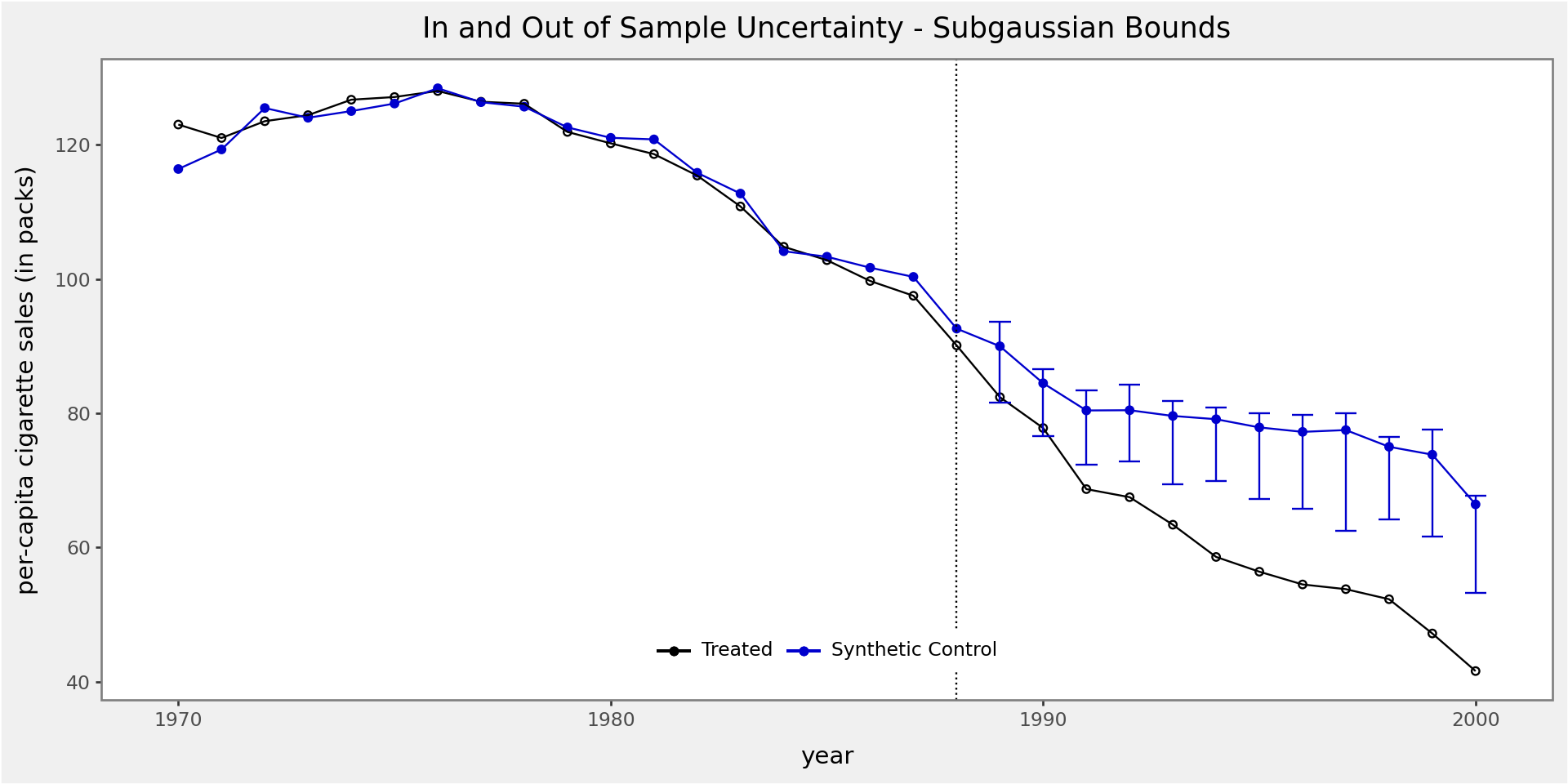
Inference
Code
from scpi_pkg.scpi import scpi
import random
w_constr = {'name': 'simplex', 'Q': 1}
u_missp = True
u_sigma = "HC1"
u_order = 1
u_lags = 0
e_method = "gaussian"
e_order = 1
e_lags = 0
e_alpha = 0.05
u_alpha = 0.05
sims = 200
cores = 1

random.seed(8894)
result = scpi(scdf, sims=sims, w_constr=w_constr, u_order=u_order, u_lags=u_lags,
              e_order=e_order, e_lags=e_lags, e_method=e_method, u_missp=u_missp,
              u_sigma=u_sigma, cores=cores, e_alpha=e_alpha, u_alpha=u_alpha)
scplot(result, e_out=True, x_lab="year", y_lab="per-capita cigarette sales (in packs)")
-----------------------------------------------
Estimating Weights...
Quantifying Uncertainty
20/200 iterations completed (10%)
40/200 iterations completed (20%)
60/200 iterations completed (30%)
80/200 iterations completed (40%)
100/200 iterations completed (50%)
120/200 iterations completed (60%)
140/200 iterations completed (70%)
160/200 iterations completed (80%)
180/200 iterations completed (90%)
200/200 iterations completed (100%)