ECON622: Computational Economics with Data Science Applications
Generalization, Deep Learning, and Representations
Overview
Summary
- Step back from optimization and fitting process to discuss the broader issues of statistics and function approximation
- Key topics:
- ERM, interpolation, and generalization error
- Features and Representations
- Neural Networks and broader hypothesis classes
- In the subsequent lecture we can briefly return to the optimization process itself to discuss
- Global vs. Local solutions
- Inductive bias and regularization
Packages
Neural Networks, Part I
Neural Networks Include Almost Everything
- Neural Networks as just an especially flexible functional form
- Linear, polynomials, and all of our standard approximation fit in there
- However, when we say “Neural Network” you should have in mind approximations that are typically
- parameterized by some complicated: \(\theta \equiv \{\theta_1, \theta_2, \cdots, \theta_L\}\)
- nested with layers: \(y = f_1(f_2(\ldots f_L(x;\theta_L);\theta_2);\theta_1) \equiv f(x;\theta)\)
- highly overparameterized, such that \(\theta\) is often massive, often far larger than the amount of data
- Terminology: depth is number of layers \(L\), width is the size of \(\theta_{\ell}\)
(Asymptotic) Universal Approximation Theorems
- At this point you may expect a theorem that says that neural networks are universal approximators. e.g., Cybenko, Hornik, and others
- i.e., for any function \(f^*(x)\), there exists a neural network \(f(x;\theta)\) that can approximate it arbitrarily well
- Takes limits of the number of parameters at each layer (e.g. \(\theta_{\ell}\nearrow\)), or sometimes the number of layers (e.g. \(L\nearrow\))
- A low bar to pass that rarely gives useful guidance or bounds
- We do not use enormously “wide” approximations
- The theorems are too pessimistic, as NNs do much better in practice
- Important when doing core functional analysis and asymptotics
How Can we Fit Huge Approximations?
- At this point you should not be scared off by a big \(\theta\)
- The ML and deep-learning revolution is built on ideas you have covered
- With a scalar loss \(L(\theta)\), you can use VJPs (reverse-mode AD) to get gradients \(\nabla_{\theta} L(\theta)\)
- AD software like PyTorch or JAX makes it easy to collect the \(\theta\) and run the AD on complicated \(L(\theta)\)
- Hardware (e.g. GPUs) can make common operations like VJPs fast
- Optimization methods like SGD work great, using gradient estimates when memory is an issue for the full \(\nabla_{\theta} L(\theta)\)
- Regularization, in all its forms, helps when used appropriately
- But that doesn’t explain why this can help generalization performance?
Puzzling Empirical Success, Ahead of Theory
- Deep learning and AD are old, but only recently have the software and hardware been good enough to scale
- Bias-variance tradeoff: adding parameters can make things worse
- But ML practitioners often find the opposite empirically
- Frequent success with lots of layers and massive over-parameterization
- This seems counter to all sorts of basic statistics intuition
- ML theory is still catching up to the empirical success
- We will try to give some perspectives on when/why deep learning works
- First, we will have to be precise on what we mean by “works”
ERM and Interpolation
Estimation and Interpolation Setup
- See ProbML Book 1 Section 5.4 on ERM
- Generalizing that notation somewhat to better nest functional equations
- Let \(p^*(x,y)\) be the true distribution on inputs \(x \in \mathcal{X}\) and outputs \(y \in \mathcal{Y}\)
- Let \(f : \mathcal{X} \to \mathcal{Y}\) be a function mapping inputs to outputs. For example, maybe \(\hat{y} = f(x)\) is an estimator for the relationship between \(x\) and \(y\) in \(p^*(x,y)\)
- For now, assume that \(f \in \mathcal{F}\) for some very large set of functions appropriate to the problem (e.g., Sobolev space, etc.)
- Define the loss as an operator \((f, x, y) \to \ell(f, x, y)\)
- For example, \(\ell(f, x, y) = (y - f(x))^2\) for LLS
Population Risk
- The population risk is then defined as
\[ R(f, p^*) \equiv \mathbb{E}_{p^*(x,y)}\left[\ell(f, x, y)\right] \]
- This lets us define the ideal minimizer of the population risk as
\[ f^{**} = \arg\min_{f \in \mathcal{F}} R(f, p^*) \]
- If \(\min_{f \in \mathcal{F}} R(f, p^*) = 0\), there is an interpolating solution across the whole of \(p^*\). Common with functional equations, rare in statistics applications
Functional Equations
- The deviations from the ProbML book are to ensure we can nest solving functional equations. In that case, we can drop the \(y\).
- We can loosely think of \(f\) as solving the functional equation as long as
\[ \min_{f \in \mathcal{F}} R(f, p^*) \equiv \min_{f \in \mathcal{F}} \mathbb{E}_{p^*(x)}\left[\ell(f, x)\right] = 0 \]
- Set the function class \(\mathcal{F}\) to be consistent with the \(\ell\)
- e.g., for \(\ell(f,x) = (\partial_x f(x) - a f(x))^2\) choose a Sobolev \(\mathcal{F}\)
- We are leaving it out here, but you might add on other terms like boundary conditions to the \(R(f,p^*)\) loss
- Note the key difference relative to standard methods is the \(p^*(x)\)!
Empirical Risk
- Denote \(N\) samples from \(p^*(x,y)\) as \(\mathcal{D} \equiv \{x_n, y_n\}_{n=1}^N\)
- We can think of this as empirical distribution \(p_{\mathcal{D}}(x,y)\)
- Which lets us define the empirical risk
\[ R(f, \mathcal{D}) \equiv \frac{1}{N}\sum_{n=1}^N \ell(f, x_n, y_n) = R(f, p_{\mathcal{D}}) \]
- Note that the empirical risk is decoupled from the function space of \(f\) and simply captures the role of finite-samples from \(p^*(x,y)\)
Hypothesis Class
- If \(\mathcal{F}\) is too large then it may be hard to solve, or we may introduce errors due to overfitting
- Instead, consider a hypothesis class \(\mathcal{H}\subseteq \mathcal{F}\), which is parameterized in practice by \(\theta \in \Theta\)
- For example, we might choose an \(\mathcal{H}\) that is a
- Linear function
- Orthogonal polynomial
- Neural network with large number of parameters and nonlinearities
Empirical Risk Minimization
- Finally, we can now look at the empirical risk minimization problem, which is the core of most statistical estimation problems like regressions
\[ f^*_{\mathcal{D}} = \arg\min_{f \in \mathcal{H}} R(f, \mathcal{D}) = \arg\min_{f \in \mathcal{H}}\frac{1}{N}\sum_{n=1}^N \ell(f, x_n, y_n) \]
- If the \(\mathcal{H}(\Theta)\), then we could implement this as
\[ \arg\min_{\theta \in \Theta} \frac{1}{N}\sum_{n=1}^N \ell(f_{\theta}, x_n, y_n) \]
Linear Least Squares
- For example, if
- \(\mathcal{H}(\Theta)\) only includes linear functions
- i.e. \(f_{\theta}(x) = \theta \cdot x\) for some \(\theta \in \Theta\)
- \(\ell(f, x, y) = (y - f(x))^2\)
- \(\mathcal{H}(\Theta)\) only includes linear functions
- Then this problem is just OLS
- \(\arg\min_{\theta \in \Theta} \frac{1}{N}\sum_{n=1}^N (y_n - \theta \cdot x_n)^2\)
- Economists are very good at analyzing the properties of the \(\mathcal{D}\) in \(p^*(x,y)\) but often ignore the differences between \(\mathcal{H}\) vs. \(\mathcal{F}\)?
- In contrast: for solving functional equations, we are better at analyzing \(\mathcal{F}\) vs. \(\mathcal{H}\), but typically implicitly assume a uniform \(p^*(x)\)
Approximation Error
- To evaluate what we lose by using \(\mathcal{H}\) instead of \(\mathcal{F}\), we can define
\[ f^* \equiv \arg\min_{f \in \mathcal{H}} R(f, p^*) \]
- Then the approximation error is defined as
\[ \varepsilon_{app}(\mathcal{H}) \equiv R(f^*, p^*) - R(f^{**}, p^*) \]
- This says, taking the population distribution as given, how close we can get a \(f^*\) to the ideal solution \(f^{**}\) using \(\mathcal{H}\) instead of \(\mathcal{F}\)
- The weighting by \(p^*(x)\) is crucial to gauge “success”
Generalization Error
- Alternatively, we can fix the hypothesis class and ask how much error we are introducing by the use of finite data \(\mathcal{D}\) instead of the population distribution \(p^*(x,y)\)
- The generalization error (or estimation error) is
\[ \varepsilon_{est}(\mathcal{H}) \equiv \mathbb{E}_{\mathcal{D} \sim p^*}\left[R(f^*_{\mathcal{D}}, \mathcal{D}) - R(f^*, p^*)\right] \]
- By that notation we are showing that this is taking the expectation over samples \(\mathcal{D}\) from the true \(p^*(x,y)\)
Calculating the Generalization Error
- Since we typically do not have the true \(p^*\), or can at most sample from it, we need to find ways to approximate the \(\varepsilon_{est}\) for a given problem.
- A typical approach is the data splitting we discussed in the previous section.
- Partition \(\mathcal{D}\) into \(\mathcal{D}_{train}\) and \(\mathcal{D}_{test}\), then solve ERM to find \[ f^*_{\mathcal{D}_{train}} = \arg\min_{f \in \mathcal{H}} R(f, \mathcal{D}_{train}) = \arg\min_{f \in \mathcal{H}}\frac{1}{N_{train}}\sum_{n=1}^{N_{train}} \ell(f, x_n, y_n) \]
- Then, we can approximate with what is sometimes called the generalization gap \[ \varepsilon_{est}(\mathcal{H}) \approx R(f^*_{\mathcal{D}_{train}} , \mathcal{D}_{train}) - R(f^*_{\mathcal{D}_{train}} , \mathcal{D}_{test}) \]
Decomposing the Error
- Armed with these definitions, we can now decompose the error of using a particular hypothesis class \(\mathcal{H}\) and finite set of samples \(\mathcal{D}\) from \(p^*\) as
\[ \mathbb{E}_{\mathcal{D} \sim p^*}\left[\min_{f \in \mathcal{H}} R(f, \mathcal{D}) - \min_{f \in \mathcal{F}} R(f, p^*)\right] = \varepsilon_{app}(\mathcal{H}) + \varepsilon_{est}(\mathcal{H}) \]
- Note that this is a property of the approximation class \(\mathcal{H}\) and the selection process for the \(\mathcal{D}\), not a particular \(\mathcal{D}\)
Tradeoffs
- This is at the core of the bias-variance tradeoff
- \(\varepsilon_{app}(\mathcal{H})\) is the bias, i.e. approximation error
- \(\varepsilon_{est}(\mathcal{H})\) is the variance, i.e. estimation error
- The classic tradeoff here is that if you make \(\mathcal{H}\) too rich, you may decrease the \(\varepsilon_{app}(\mathcal{H})\) but the extra flexibility may lead to a much higher \(\varepsilon_{est}(\mathcal{H})\)
- i.e., flexibility leads to overfitting
- In the next lectures we will investigate this classic intuition in more detail and discuss when it falls apart.
- Hint: consider the role of regularization in all its forms
- The bigger challenge is that as data and economic mechanisms become richer, you may not be able to choose the appropriate \(\mathcal{H}\) manually
Features and Representations
Features
- The features of a problem start with the inputs that we use within the hypothesis class \(\mathcal{H}(\Theta)\)
- Economists are used to shallow approximations, e.g.,
- Linear functions, \(f_{\theta}(x) = \theta \cdot x\)
- Orthogonal polynomials, \(f_{\theta}(x) = \sum_{m=1}^M \theta_m \phi_m(x)\) for basis \(\phi_m(x)\)
- Economists feature engineer to choose the appropriate \(x\in\mathcal{X}\) form raw data, typically then used with shallow approximations
- e.g. log, dummies, polynomials, first-differences, means, etc.
- Embeds all sorts of priors, wisdom, and economic intuition
- Priors are inescapable - and a good thing as long as you are aware when you use them and how they affect inference
Simple Representation in ERM
To abstract from this manual process, we can think of instead taking the raw data \(x\) and transforming it into a representation \(z\in \mathcal{Z}\) with \(g : \mathcal{X} \to \mathcal{Z}\)
Then, instead of finding a \(f : \mathcal{X} \to \mathcal{Y}\), we can find a \(\tilde{f} : \mathcal{Z} \to \mathcal{Y}\) and in our loss use \(\ell(\tilde{f}\circ g, x, y)\)
\[ \tilde{f}^*_{\mathcal{D}} = \arg\min_{\tilde{f} \in \mathcal{H}}\frac{1}{N}\sum_{n=1}^N \ell(\tilde{f} \circ g, x_n, y_n) \]
- And then define \(f^*_{\mathcal{D}} \equiv \tilde{f}^*_{\mathcal{D}} \circ g\)
Our approximation class \(\mathcal{H}\) then changes - for better or worse.
Finding Representations is an Art
- This is the process of finding latent variables and inverse mapping from observables to them
- What is our goal when choosing \(g\)?
- Drop irrelevant information, which is the simplest feature engineering
- Find \(z\) that captures the relevant information in \(x\) for the problem at hand (i.e., the particular \(\ell, y, \mathcal{D}\))
- See ProbML Book 2 Section 5.6 for more on information theory
- Disentangled (i.e., the factors of variation are separated out in \(z\))
Problem Specific or Reusable?
- Are representations reusable between tasks?
- e.g., our wisdom of when to take logs or first-differences is often reusable
- Remember: representations are on \(\mathcal{X}\), not \(\mathcal{Y}\)
- Encodes age old wisdom from working with the datasources
- Though wisdom probably included seeing \(\mathcal{Y}\) from previous tasks
- What if \(\mathcal{X}\) is complicated, or we are worried we may have chosen the wrong \(z = g(x)\)?
- Can we learn this automatically?
Can Representations Be Learned?
- The short answer is: yes, but it is still an art (with finite data)
- Representation learning finds representations \(g : \mathcal{X} \to \mathcal{Z}\) using \(\mathcal{D}\)
- Hopefully: works well for \(x \sim p^*(x,y)\), and for many \(\ell(\tilde{f} \circ g, x, y)\)
- This happens in subtle ways in many different methods. e.g.
- If we run “unsupervised” clustering or embeddings on our data to embed it into a lower dimensional space then run a regression
- “Learning the kernel”. See ProbML Book 2 Section 18.6
- Autoencoders and variational autoencoders
- Deep learning approximations, which we will discuss in detail
Benefits of Having Learned Representations
- If you know the correct features, there is no benefit besides maybe dimension reduction. But are you so sure they are correct?
- Can handle complicated data (e.g. text, networks, high-dimensions)
- Maybe the representations are reusable across problems, just like they were for our manual feature engineering
- This is part of the process of transfer learning and fine-tuning
- Using a good representation is more sample efficient because data ends up used in fitting \(\tilde{f}\) instead of jointly finding \(f = \tilde{f} \circ g\)
- Maybe problems which are complicated and nonlinear in \(\mathcal{X}\) are simpler in \(\mathcal{Z}\) (i.e., linear regression in \(\mathcal{Z}\))
- Above all: good representations overfit less and generalize better
Jointly Learning Representations and Functions?
- Because \(f \equiv \tilde{f} \circ g\), the simplest approach is just to jointly learn both
- Come up with some hypothesis class \(\mathcal{H}\) that flexible enough to have both the representation and function of interest
- Extra flexibility could overfit (i.e., \(\varepsilon_{est}(\mathcal{H})\) could increase even if \(\varepsilon_{app}(\mathcal{H}) \searrow 0\))
- Hence the crucial need for regularization in various forms
- Notice the nested structure here of \(\tilde{f} \circ g\)
- Hints at why Neural Networks might work so well
Is this a Mixture of Supervised and Unsupervised?
- Remember that we talked about finding representations as intrinsic to the data itself, and hence “unsupervised”
- Fitting \(\tilde{f} \circ g\) jointly combines supervised and unsupervised
- Nested structure means we may be able to use this for new problems
- Isolate the \(g\) parameters and structure from the \(\tilde{f}\)
- Train \(\tilde{f} \circ g\) for a new \(\tilde{f}\) and fit jointly again or freeze the \(g\)
- Can work shockingly well in practice!
- What do Neural Networks Learn When Trained on Random Labels?
- Best to start with existing representations and fine-tune (essential in LLMs)
Neural Networks, Part II
Rough Intuition on The Success of Deep Learning
- The broadest intuition on why deep learning with flexible, overparameterized neural networks often works well is a combination of:
- The massive number of parameters makes the optimization process find more generalizable solutions (sometimes through regularization)
- The depth of approximations allowing for better representations
- The optimization process seems to be able to learn those representations
- The representations are reusable across problems
- Regularization (implicit and explicit) helps us avoid overfitting
- Art, not magic
- Need to design architectures (\(\mathcal{H}\)), optimization, and regularization
Neural Networks and Representations
- Neural networks are typically “deep”: \(f_1(f_2(\ldots f_L(x;\theta_L);\theta_2);\theta_1) \equiv f(x;\theta)\)
- If we fit \(f(x) \equiv \tilde{f}(g(x;\theta_1);\theta_2)\) then there is a chance that we could fit both a good representation and a generalizable function
- So it seems that having two “layers” helps. What is less clear is that
- Having further nesting of representations helps
- That the representations themselves can be learned in this way
- For examples on why multiple layers help see:Mark Schmidt’s CPSC 440, CPSC340, ProbML Book 1 Section 13.2.1 on the XOR Problem and 13.2.5-13.2.7 for more
Common Neural Network Designs
- A common pattern for \(\mathcal{H}\) is called the Multi Layer Perception (MLP)
- See ProbML Book 1 Section 13.2
- Alternate linear/nonlinear then end with linear (or match domain)
- One hidden layer \(f(x) = W_2 \sigma(W_1 x + b_1) + b_2\)
- Another layer: \(f(x) = W_3 \sigma(W_2 \sigma(W_1 x + b_1) + b_2) + b_3\)
- Where \(\sigma(\cdot)\) is a nonlinear activation function in the jargon. e.g. \(\tanh(\cdot)\) or \(\max(0, \cdot)\) (called ReLU)
- See ProbML Book 1 Section 13.2.4 numerical properties of gradients
- If \(f : \mathbb{R}^N \to \mathbb{R}\) with 2 hidden layers and width of \(M\):
- \(W_1 \in \mathbb{R}^{M \times N}, b_1 \in \mathbb{R}^M, W_2 \in \mathbb{R}^{M \times M}, b_2 \in \mathbb{R}^M, W_3 \in \mathbb{R}^{1 \times M}, b_3 \in \mathbb{R}\)
Many Problem Specific Variations
Use economic intuition and problem specific knowledge to design \(\mathcal{H}\)
- Encode knowledge of good representations, easier learning
For example, you can approximation function \(f : \mathbb{R}^N \to \mathbb{R}\) which are symmetric in arguments (i.e. permutation invariance) with
\[ f(X) = \rho\left(\frac{1}{N}\sum_{x\in X} \phi(x)\right) \]
- \(\rho : \mathbb{R}^M \to \mathbb{R}\), \(\phi : \mathbb{R} \to \mathbb{R}^M\) both neural networks
See Probabilistic Symmetries and Invariant Neural Networks or Exploiting Symmetry in High Dimensional Dynamic Programming
Transfer Learning and Few-Shot Learning
- If you have a good representation, you can often use it for new problems
- Take the \(\theta\) as an initial condition for the optimizer and fine-tune on the new problem
- e.g. take \(g \equiv f_1 \circ f_2 \circ \ldots f_{L-1}\) (e.g. the all but the last layer) and freeze them only changing the last \(f_L\) layer with training
- Or only freeze some of them
- May work well even if the task was completely different. Many \(y\) $are simply linear combinations of the disentangled representations - part of why kernel methods (which we will discuss in a future lecture) work well
- Can find sometimes “one-shot”, “few-shot”, or “zero-shot” learning
- e.g. Zero-Shot Learning for image classification
More Perspectives on Representations
The Tip of the Iceberg
- The ideas sketched out previously are just the beginning
- This section points out a few important ideas and directions for you to explore on your own
Autoencoders and Representations
- One unsupervised approach is to consider autoencoders. See ProbML Book 1 Section 20.3, ProbML Book 2 Section 21, and CPSC 440 Notes
- Consider connection between representations and compression
- Let \(g : \mathcal{X} \to \mathcal{Z}\) be a encoder and \(h : \mathcal{Z} \to \mathcal{X}\) be a decoder, parameterized by some \(\theta_d\) and \(\theta_e\) then we want to find the empirical equivalent to
\[ \min_{\theta_e, \theta_d} \mathbb{E}_{p^*(x)} (h(g(x;\theta_e);\theta_d) - x)^2 + \text{regularizer} \]
- Whether the \(g(x;\theta_e)\) is a good representation depends on whether “compression” of the information of \(x\) is useful for downstream tasks
Manifold Hypothesis
- Are there always simple, reusable representations?
- On perspective is called the Manifold Hypothesis, see ProbML Book 1 Section 20.4.2
- The basic idea is that even the most complicated data sources in the real world ultimately are concentrated on a low-dimensional manifold
- including images, text, networks, high-dimensional time-series, etc.
- i.e., the world is much simpler than it appears if you find the right transformation
- See ProbML Book 1 Section 20.4.2.4 describes Manifold Learning, which tries to learn the geometry of these manifolds through variations on nonlinear dimension reduction
Embeddings
- A related idea is to embed data into a different (sometimes lower-dimensional) space
- For example, text or images or networks, mapped into \(\mathbb{R}^M\)
- Whether it is lower or higher dimensional, the key is to preserve some geometric properties, typically a norm. i.e., \(||x - y|| \approx ||g(x) - g(y)||\)
- You can think of learned representations within the inside of neural networks as often doing embedding in some form, especially if you use an information bottleneck
- See ProbML Book 1 Section 20.5 and 23 for examples with text and networks
Lottery Tickets and Representations
- The Lottery Ticket Hypothesis: Finding Sparse, Trainable Neural Networks
- The idea is that inside of every huge, overparameterized approximation with random initialization and layers is a small sparse approximation
- You can show this by pruning most of the parameters and training it
- Perhaps huge, overparameterized functions with many layers are more likely to contain the lottery ticket
- Then the optimization methods are just especially good at finding them
- Ex-post you could prune, but ex-ante you don’t know the sparsity structure
Distentangling Representations
- Representations that separate out different factors of variation into separate variables are often easier to use for downstream tasks and are more transferrable
- The keyword in a literature review is to look for is disentangled representations
- It seems like this is hard to do without supervision
- But semi-supervised approaches seem to be a good approach
Out of Distribution Learning
- We have been discussing a \(\mathcal{D}\) from some idealized, constant \(p^*(x,y)\)
- What if the distribution changes, or our samples are not IID. e.g., in control and reinforcement learning applications where it is \(p^*(x,y;f)\)?
- See ProbML Book 2 Section 19.1 for more
- This is called “robustness to distribution shift”, covariate shift, etc. in different settings
- There are many methods, but one common element is:
- Models with better “generalization” tends to perform much better under distribution shift
- Good representations are much more robust
- With transfer learning you may be able to adapt very easily
Differentiating Representations
Recursive Parameterizations
- \(\mathcal{H}\) design is crucial, and we can use economic intuition to guide
- If we are using ``deep’’ learning - where the representations themselves must be learned, then there will recursively defined, nested approximations
- Each of these approximations has its own parameters
- When a gradient is taken in the optimizing process, it is taken with respect to that recursive set of parameters
- ML frameworks like Pytorch, Keras, and Flax NNX help keep track of those nested parameters, update gradients, etc.
Flax NNX Example
- We previously say how to create our own
MyLinearcase for a linear function without an affine term (i.e., no “bias”) - The “learnable” (i.e, differentiable) parameters are tagged with
nnx.Param
Differentiation With Respect to nnx.Module
- Differentiating
MyLinearit finds thennx.Param. - The return thype of
nnx.graddoes not perturbout_size, etc.
State({
  'kernel': VariableState(
    type=Param,
    value=Array([[-1.5557193, -0.8495713, -1.1160917]], dtype=float32)
  )
})
Nesting
- This recursively goes through any
nnx.Module - Using the built-in
nnx.Linearinstead, construct a simple NN
class MyMLP(nnx.Module):
    def __init__(self, din, dout, width: int, *, rngs: nnx.Rngs):
        self.width = width
        self.linear1 = nnx.Linear(din, width, use_bias = False, rngs=rngs)
        self.linear2 = nnx.Linear(width, dout, use_bias = True, rngs=rngs)

    def __call__(self, x: jax.Array):
        x = self.linear1(x)
        x = nnx.relu(x)
        x = self.linear2(x)
        return x
m = MyMLP(N, 1, 2, rngs = rngs)
Reverse-mode AD
- Consider the JVP
f(m). Recall notation in Differentation lecture - For forward mode, we perturb \(f(m)\) and calculate \[ \partial f(m)^{\top}[\dot{f}] = \dot{f} \cdot \nabla f(m) \]
- Given \(f : \mathcal{H} \to \mathbb{R}\), the natural adjoint vector is \(\dot{f} = 1\)
- This is what the
jax.graddoes, for scalar functions
- This is what the
- The
nnx.graddoes this, recursively going through eachnnx.Moduleand itsnnx.Paramvalues
Splitting into Differentiable Parts
State({
  'linear1': {
    'bias': VariableState(
      type=Param,
      value=None
    ),
    'kernel': VariableState(
      type=Param,
      value=Array([[-0.11148886,  0.66866976],
             [-0.09731744, -0.486882  ],
             [-0.9420541 , -0.13140532]], dtype=float32)
    )
  },
  'linear2': {
    'bias': VariableState(
      type=Param,
      value=Array([0.], dtype=float32)
    ),
    'kernel': VariableState(
      type=Param,
      value=Array([[-0.1044913 ],
             [-0.18319812]], dtype=float32)
    )
  }
})
graphdef Contains Fixed Values and Metadata
GraphDef(
  nodedef=NodeDef(
    type=MyMLP,
    index=0,
    attributes=('linear1', 'linear2', 'width'),
    subgraphs={
      'linear1': NodeDef(
        type=Linear,
        index=1,
        attributes=('bias', 'bias_init', 'dot_general', 'dtype', 'in_features', 'kernel', 'kernel_init', 'out_features', 'param_dtype', 'precision', 'use_bias'),
        subgraphs={
          'dtype': NodeDef(
            type=PytreeType,
            index=-1,
            attributes=(),
            subgraphs={},
            static_fields={},
            leaves={},
            metadata=PyTreeDef(None)
          ),
          'precision': NodeDef(
            type=PytreeType,
            index=-1,
            attributes=(),
            subgraphs={},
            static_fields={},
            leaves={},
            metadata=PyTreeDef(None)
          )
        },
        static_fields={
          'bias_init': <function zeros at 0x0000026AE86D0E00>,
          'dot_general': <function dot_general at 0x0000026AE8187060>,
          'in_features': 3,
          'kernel_init': <function variance_scaling.<locals>.init at 0x0000026AF2993740>,
          'out_features': 2,
          'param_dtype': <class 'jax.numpy.float32'>,
          'use_bias': False
        },
        leaves={
          'bias': 2,
          'kernel': 3
        },
        metadata=<class 'flax.nnx.nnx.nn.linear.Linear'>
      ),
      'linear2': NodeDef(
        type=Linear,
        index=4,
        attributes=('bias', 'bias_init', 'dot_general', 'dtype', 'in_features', 'kernel', 'kernel_init', 'out_features', 'param_dtype', 'precision', 'use_bias'),
        subgraphs={
          'dtype': NodeDef(
            type=PytreeType,
            index=-1,
            attributes=(),
            subgraphs={},
            static_fields={},
            leaves={},
            metadata=PyTreeDef(None)
          ),
          'precision': NodeDef(
            type=PytreeType,
            index=-1,
            attributes=(),
            subgraphs={},
            static_fields={},
            leaves={},
            metadata=PyTreeDef(None)
          )
        },
        static_fields={
          'bias_init': <function zeros at 0x0000026AE86D0E00>,
          'dot_general': <function dot_general at 0x0000026AE8187060>,
          'in_features': 2,
          'kernel_init': <function variance_scaling.<locals>.init at 0x0000026AF2993740>,
          'out_features': 1,
          'param_dtype': <class 'jax.numpy.float32'>,
          'use_bias': True
        },
        leaves={
          'bias': 5,
          'kernel': 6
        },
        metadata=<class 'flax.nnx.nnx.nn.linear.Linear'>
      )
    },
    static_fields={
      'width': 2
    },
    leaves={},
    metadata=<class '__main__.MyMLP'>
  ),
  index_mapping=None
)
Differentiation with Nested nnx.Module
State({
  'linear1': {
    'bias': VariableState(
      type=Param,
      value=None
    ),
    'kernel': VariableState(
      type=Param,
      value=Array([[-0.784888  , -2.226523  ],
             [-0.42862383, -1.2158941 ],
             [-0.5630881 , -1.5973343 ]], dtype=float32)
    )
  },
  'linear2': {
    'bias': VariableState(
      type=Param,
      value=Array([1.], dtype=float32)
    ),
    'kernel': VariableState(
      type=Param,
      value=Array([[0.97357047],
             [1.0623739 ]], dtype=float32)
    )
  }
})
Interpreting the “Adjoint”
- This gradient is a recursive structure for a change in the object linearized around the value \(m\)
- Note that this is a \(\delta m\) for the state, and ignores the
graphdef - Crucially, we need to do the operation like \(m - \eta \,\delta m\) to update the parameters, keeping fixed all of the non-differentiable parts
- The optimization process with find the update wrt the state, apply it, and then reconstruct the new
mby applying the graphdef
Split and Merge
- In that case, we can update the
statefrom before, and make a new type using thegraphdef
eta = 0.01 # e.g., a gradient descent update

# jax.tree.map recursively goes through the model
# Updates the underlying nnx.Param given the delta_m grad
new_state = jax.tree.map(
  lambda p, g: p - eta*g,
  state, delta_m) # new_state = state - eta * delta_m
m_new = nnx.merge(graphdef, new_state)
f(m_new)
Array(0.84317195, dtype=float32)Manually Splitting and Merging
- The
nnx.jit, nnx.vmap, nnx.gradwill automatically split and merge for you (i.e., filtering) onnnx.Moduletypes as arguments, then call underlying JAX functions- Otherwise the
nnx.gradetc. would not work without modification since the NN combine differentiable and non-differentiable parts
- Otherwise the
- There is some overhead. You can manually split into the
stateandgraphdefand then merge them back together - Next we will show that process with a different wrapper for the
f_genfunction
Functions of the state
graphdef, state = nnx.split(m)
@jax.jit # note jax.jit instead of nnx.jit
def f_split(state): # closure on graphdef
    m = nnx.merge(graphdef, state)
    return f_gen(m, x, b)
# Can use jax.grad, rather than nnx.grad
state_diff = jax.grad(f_split)(state)
print(state_diff)
new_state = jax.tree.map(
            lambda p, g: p - eta*g,
            state, delta_m)
m_new = nnx.merge(graphdef, new_state)
f(m_new)
State({
'linear1': {
'bias': VariableState(
type=Param,
value=None
),
'kernel': VariableState(
type=Param,
value=Array([[-0.784888 , -2.226523 ],
[-0.42862383, -1.2158941 ],
[-0.5630881 , -1.5973343 ]], dtype=float32)
)
},
'linear2': {
'bias': VariableState(
type=Param,
value=Array([1.], dtype=float32)
),
'kernel': VariableState(
type=Param,
value=Array([[0.97357047],
[1.0623739 ]], dtype=float32)
)
}
})Array(2.8807144, dtype=float32)Pytorch (and Functorch)
- The gradients of structures in JAX are more explicit, as the functions are generally pure (i.e., side-effect free)
- Pytorch, on the other hand, implicitly does these same operations in the background.
- This can lead to concise code, but can also lead to confusion
- torch.func is a Torch library intended for more JAX-style function composition
Pytorch Custom Types
- The equivalent to
nnx.Paramin Pytorch istorch.nn.Parameter
class MyLinearTorch(nn.Module):
    def __init__(self, in_size, out_size):
        super(MyLinearTorch, self).__init__()
        self.out_size = out_size
        self.in_size = in_size
        self.kernel = nn.Parameter(torch.randn(out_size, in_size))
        # Similar to PyTorch's forward
    def forward(self, x):
        return self.kernel @ x
def f_gen_torch(m, x, b):
    return torch.squeeze(m(x) + b)
Differentiating Modules in Pytorch
Parameter containing:
tensor([[-0.6374, -0.7554,  0.5486]], requires_grad=True)
Differentiating Custom Types
class MyMLPTorch(nn.Module):
    def __init__(self, din, dout, width):
        super(MyMLPTorch, self).__init__()
        self.width = width
        self.linear1 = nn.Linear(din, width, bias=False)
        self.linear2 = nn.Linear(width, dout, bias=True)

    def forward(self, x):
        x = self.linear1(x)
        x = torch.relu(x)
        x = self.linear2(x)
        return x
Reverse-mode AD Updates in Pytorch
m = MyMLPTorch(N, 1, 2)
m.zero_grad()
output = f_torch(m)

# Start with d output = [1.0]
output.backward()
# Now `m` has the gradients

# Manually update parameters recursively
# Done in-place, as torch optimizers will do
with torch.no_grad():
    # Recursively
    for param in m.parameters():
        param -= eta * param.grad
    for name, param in m.named_parameters():
        print(f"{name}: {param.numpy()}")
linear1.weight: [[ 0.340191 0.4308803 0.16260189]
[-0.07866785 -0.35180938 0.44592345]]
linear2.weight: [[ 0.2432586 -0.7069635]]
linear2.bias: [-0.41789627]Hyperparameter Optimization with Deep Learning
Optimization is Challenging
- When using complicated representations, we often have many fixed values (e.g. the
width) of the representations, as well as tweaks to the optimizer and algorithms - Collectively we call the values not found through differentiation of the representations themselves hyperparameters
- When possible, you should use optimizers to find these in a systematic way (i.e., differentiating the solution to the optimizer itself)
- But often you need to do this manually through a combination of brute force, intuition, and experience
Commandline Arguments
Given that you may want to solve your problem with a variety of different hyperparameters, possibly running in parallel, you need a convenient way to pass the values and see the results
One model, framework, OS independent way to do this is to use commandline arguments
For example, if you have a python file called
mlp_regression_jax_nnx_logging.pythat accepts arguments for the width and learning rate, you may call it with
CLI Packages
Many python frameworks exist to help you take CLI and convert to calling python functions. One convenient tool isjsonargparse
Advantage: simply annotate a function with defaults, and it will generate the CLI
Then can call
python mlp_regression_jax_nnx_logging.py,python mlp_regression_jax_nnx_logging.py --width=64etc.
Logging
While the CLI file could save output for later interpretation, a common approach in ML is to log results to visualize the optimization process, compare results, etc.
One package for this is Weights and Biases
This will log into a website calculations, usually organized by a project name, and let you sort hyperparameters, etc.
To use this, setup an account and then add code to initialiize in your python file, then log intermediate results
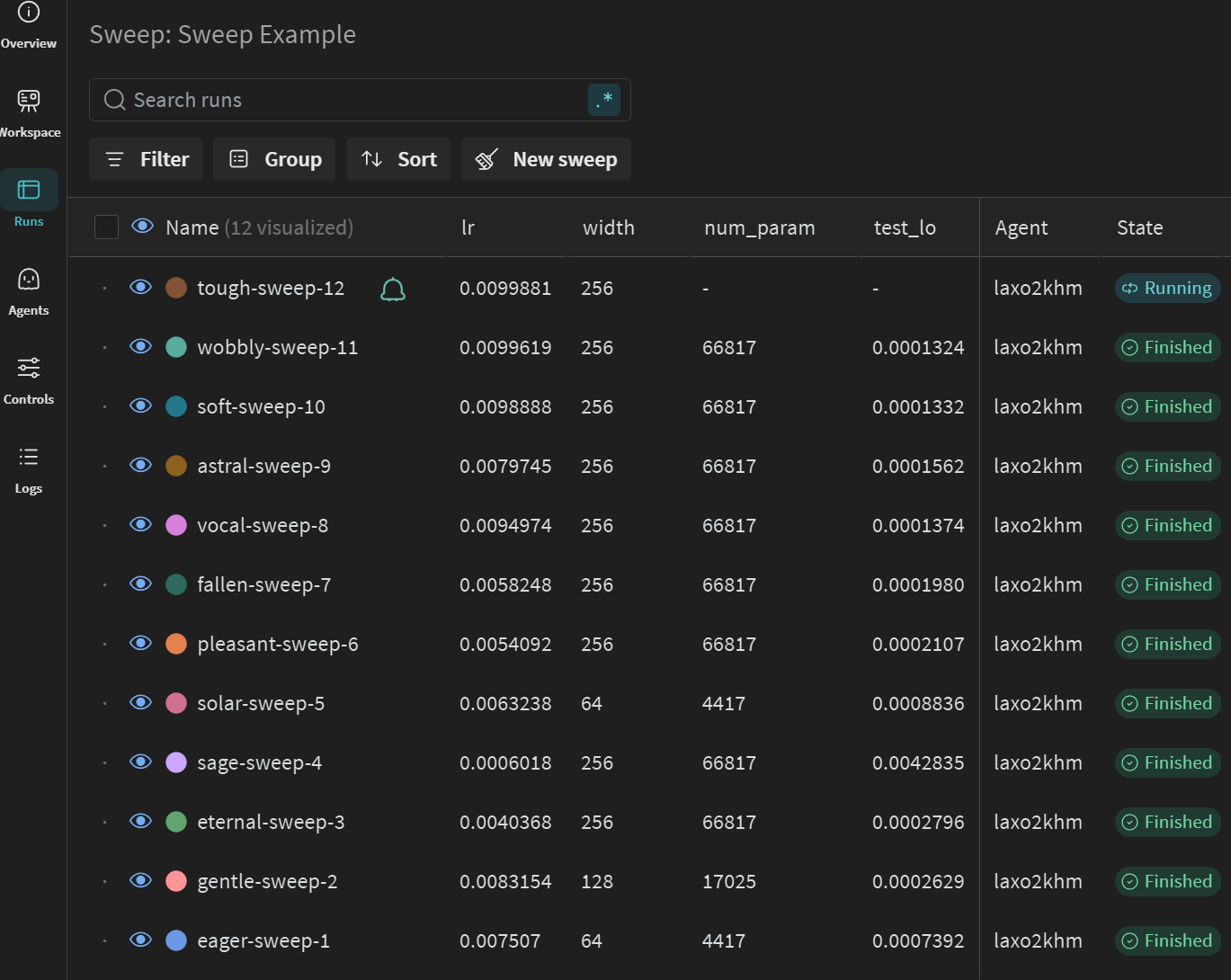
HPO “Sweeps” with Weights and Biases
Putting together the logging and the CLI, you can setup a process to run the code with a variety of parameters in a “sweep” (e.g., with sweep file)
- Returns a sweep ID, which you can then run with
wandb agent <sweep_id> - Which calls function given instructions (i.e., polling architecture)
python mlp_regression_jax_nnx_logging.py --width=128 --lr=0.0015etc. - Benefit: run with same
<sweep_id>on multiple computers/processes/etc.
- Returns a sweep ID, which you can then run with
Example Sweep File
- Sets up a Bayesian optimization process on
lrandwidthto minimizetest_loss(if logged withwandb.log({"test_loss": test_loss}), etc.)
program: lectures/examples/mlp_regression_jax_nnx_logging.py
name: Sweep Example
method: bayes
metric:
  name: test_loss
  goal: minimize
parameters:
  num_epochs:
    value: 300 # fixed for all calls
  lr: # uniformly distributed
    min: 0.0001
    max: 0.01
  width: # discrete values to optimize over
    values: [64, 128, 256]
MLP Regression Example with Sweep
MLP Regression
- See examples/mlp_regression_jax_nnx_logging.py for an example of a simple neural network optimized to fit a linear DGP
- The \(\mathcal{H}\) is a simple nesting of
nnx.Linearandnnx.relulayers
class MyMLP(nnx.Module):
    def __init__(self, din: int, dout: int, width: int, *, rngs: nnx.Rngs):
        self.linear1 = nnx.Linear(din, width, rngs=rngs)
        self.linear2 = nnx.Linear(width, width, rngs=rngs)
        self.linear3 = nnx.Linear(width, dout, rngs=rngs)

    def __call__(self, x: jax.Array):
        x = self.linear1(x)
        x = nnx.relu(x)
        x = self.linear2(x)
        x = nnx.relu(x)
        x = self.linear3(x)
        return x
Data Generating Process and Loss
This randomly generates a \(\theta\) and then generates data with
ERM: with \(m \in \mathcal{H}\), minimize the residuals for batch
(X, Y)Optimizer uses loss differentiated wrt \(m\) as discussed
CLI
In order to use
jsonargparse, this creates a function signature with defaultsdef fit_model( N: int = 500, M: int = 2, sigma: float = 0.0001, width: int = 128, lr: float = 0.001, num_epochs: int = 2000, batch_size: int = 512, seed: int = 42, wandb_project: str = "econ622_examples", wandb_mode: str = "offline", # "online", "disabled ): # ... generate data, fit model, save test_loss
Sweep File
Run and Visualize the Sweep
To run this sweep, you can run the following command (checking the relative location file)
The output should be something along the lines of
(econ622) C:\Users\jesse\Documents\GitHub\ECON622_instructor>wandb sweep lectures/examples/mlp_regression_jax_nnx_sweep.yaml
wandb: Creating sweep from: lectures/examples/mlp_regression_jax_nnx_sweep.yaml
wandb: Creating sweep with ID: virfdcn6
wandb: View sweep at: https://wandb.ai/highdimensionaleconlab/ECON622_instructor-lectures_examples/sweeps/virfdcn6
wandb: Run sweep agent with: wandb agent highdimensionaleconlab/ECON622_instructor-lectures_examples/virfdcn6- Run
wandb agent highdimensionaleconlab/ECON622_instructor-lectures_examples/virfdcn6and go to web to see results in progress
General Sweep Results
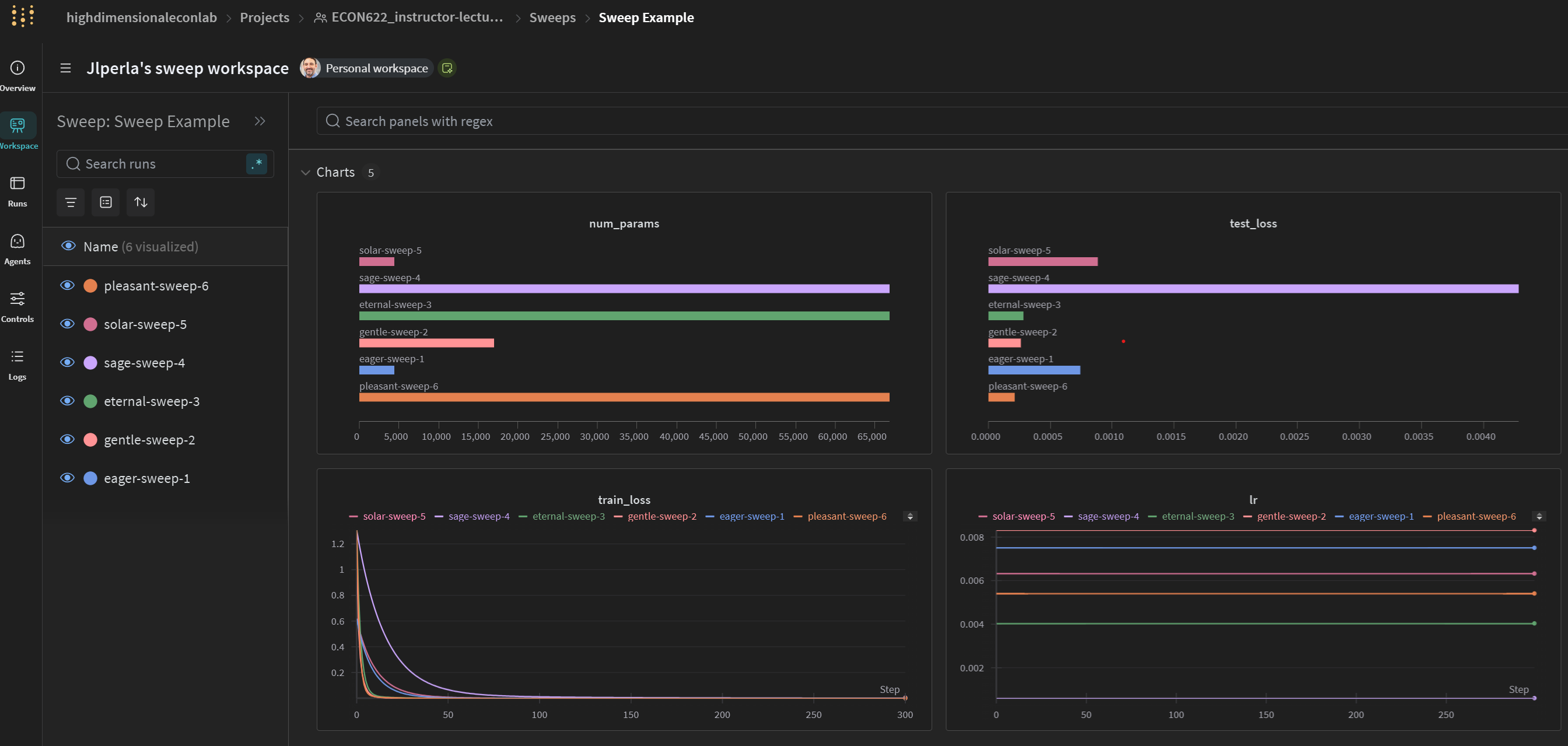
Correlations of Parameters to HPO Objective
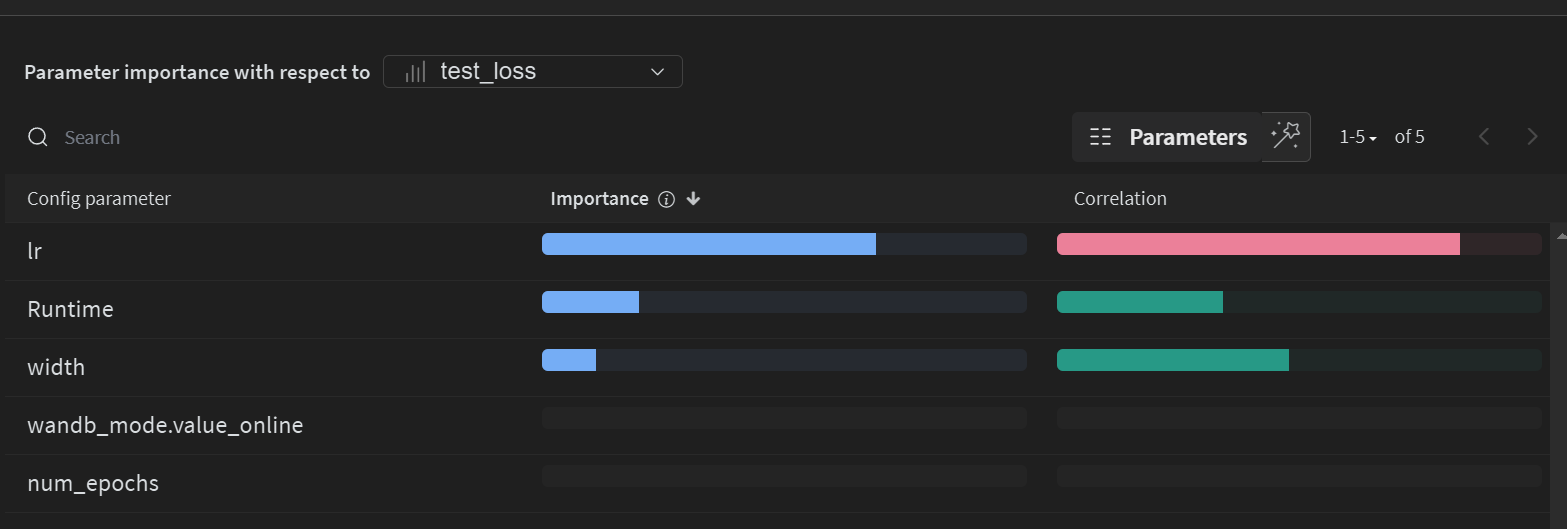
Sortable Table of Results