Linear Algebra

UBC Economics Math Camps

Jesse Perla

William Duan

Table of contents

• Introduction
• Vectors
• Orthogonality and Linear Independence
• Matrices
• Matrix Inverse and Systems
• PhD MaterialPhD
• Matrices as DataPhD
• ProjectionPhD
• The Structure of \(X'X\)PhD
• Quadratic Forms and DefinitenessPhD

Lecture Videos

• Vectors and Linear Combinations
• Matrices and Systems of Equations

Introduction

Matrix and Linear Algebra

• In this section we will review basic operations and matrix algebra and concepts
• In ECON526 we will be using a computer for most computations, but the basic theory will be important to understanding topics such as identification
• Practice questions at the end of the notes will be discussed in the review session

• You can never know too much linear algebra
• Even though modern ML seems like it is highly non-linear and abstract, it is often based on linearizations under the hood.

Vectors

Vectors

• Notation: \(x \in \mathbb{R}^{n}\) is a vector of \(n\) reals (i.e., \(\mathbb{R}\))
• Vector \(x = \begin{bmatrix} x_1 \\ x_2 \\ \vdots \\ x_n\end{bmatrix}\)
• Element: \(x_i\) is the \(i\)th element of the vector \(x\)

Vector Addition

• Definition: \((x + y)_i = x_i + y_i\)
• Example: \(\begin{bmatrix} 1 \\ 2 \\ 3 \end{bmatrix} + \begin{bmatrix} 4 \\ 5 \\ 6 \end{bmatrix} = \begin{bmatrix} 5 \\ 7 \\ 9 \end{bmatrix}\)

Vector Scalar Multiplication

• Definition: \((\alpha x)_i = \alpha x_i\) for \(\alpha \in \mathbb{R}\)
• Commutative: \(\alpha x = x \alpha\)
• Example: \(2 \times \begin{bmatrix} 1 \\ 2 \\ 3 \end{bmatrix} = \begin{bmatrix} 2 \\ 4 \\ 6 \end{bmatrix}\)

Inner Product

• The dot product (also called the inner product) of two vectors \(x, y \in \mathbb{R}^n\) is defined as

\[ x \cdot y = \sum_{i=1}^n x_i y_i \]

• Properties:
  • Commutative: \(x \cdot y = y \cdot x\)
  • Distributive: \(x \cdot (y + z) = x \cdot y + x \cdot z\)
  • Scalar multiplication: \((\alpha x) \cdot y = x \cdot (\alpha y) = \alpha (x \cdot y)\) for \(\alpha\in\mathbb{R}\)

• If, for example, you had a vector of coefficients \(\beta\) and data \(x\) then the prediction in OLS might be \(\beta \cdot x\)
• Properties: \(x \cdot(y + \alpha z) = \alpha x \cdot(1/\alpha y + z) = x \cdot y + \alpha x \cdot z = y \cdot x + \alpha z \cdot x\)
• In econometrics and ML, these may be more abstract types of objects—e.g., functions.
  • Later we will look at some interpretations of inner products as measures of similarity.

Inner Product Example

• \(x = \begin{bmatrix} 1 \\ 2 \\ 3 \end{bmatrix}\) and \(y = \begin{bmatrix} 4 \\ 5 \\ 6 \end{bmatrix}\), then

\[ x \cdot y = (1 \times 4) + (2 \times 5) + (3 \times 6) = 32 \]

Euclidean Norm

• The Euclidean norm of a vector \(x \in \mathbb{R}^n\) is defined as

\[ \|x\|_2 = \sqrt{\sum_{i=1}^n x_i^2} \]

• Or defined using the inner product: \(\|x\|_2 = \sqrt{x \cdot x}\)
• Often will use the square of the norm: \(\|x\|_2^2 = x \cdot x\)
• Distance from origin: \(x = \begin{bmatrix} 2 & 0\end{bmatrix}, y = \begin{bmatrix} 0 & 2 \end{bmatrix}, z = \begin{bmatrix} -2 & 0\end{bmatrix}\) then \(\|x\|_2 = \|y\|_2 = \|z\|_2 = \sqrt{4} = 2\)

What Remains Invariant

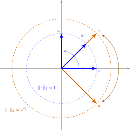
• Vectors of the same norm lie on the same circle
• “Reflections” preserve the length
  • \(x = \begin{bmatrix} 1 & 1\end{bmatrix}\), \(y = \begin{bmatrix} 1 & -1\end{bmatrix}\)
  • \(\|x\|_2 = \|y\|_2 = \sqrt{2}\)
• “Rotations” preserve the length
  • \(u = \begin{bmatrix} 0 & 1\end{bmatrix}\), \(v = \begin{bmatrix} 1 & 0\end{bmatrix}\), \(w = \begin{bmatrix} \tfrac{1}{\sqrt{2}} & \tfrac{1}{\sqrt{2}}\end{bmatrix}\)
  • \(\|u\|_2 = \|v\|_2 = \|w\|_2 = 1\)
• Unit length if \(\|x\|_2 = 1\)

• Every arrow ending on the same dashed circle has the same norm: the circle is the set of all vectors of that length
• Rotations sweep along the circle, reflections flip across a line (here the \(x_1\) axis) — neither changes the norm
• The previous slide’s \((2,0), (0,2), (-2,0)\) all sit on the circle of radius \(2\)

Other Norms

• Many norms providing different interpretations of “length”
• \(L_1\) norm: \(\|x\|_1 = \sum_{i=1}^n |x_i|\)
• \(L_\infty\) norm: \(\|x\|_\infty = \max_{i=1,\ldots,n} |x_i|\)
• If just \(\|x\|\), assume Euclidean norm by default (i.e., \(\|x\|_2\))

• Could show in the picture that the set of all points with \(L_1\) norm 1 is a diamond, and the set of all points with \(L_\infty\) norm 1 is a square (in contrast to the circle for the Euclidean norm)
• In all cases, the norm goes through the corners at \((1,0), (0,1), (-1,0), (0,-1)\)

Orthogonality and Linear Independence

Interpretations of Inner Product

• \(x \cdot y\) gives a sense of the “angle” between the vectors
• If \(x \cdot y = 0\) then the vectors are orthogonal (i.e., at right angles)
  • e.g., if \(x = \begin{bmatrix} 1 & 0\end{bmatrix}, y = \begin{bmatrix} 0 & 1\end{bmatrix}\) then \(x \cdot y = 0\).
  • Invariant to scale: \(x = \begin{bmatrix} 2 & 0\end{bmatrix}, y = \begin{bmatrix} 0 & 1\end{bmatrix}\) then \(x \cdot y = 0\)
• If \(x\) and \(y\) are of the same length (\(\|x\|_2 = \|y\|_2\)), then \(x \cdot y\) measures the similarity. important applications in ML/datascience
  • If \(x\) and \(y\) are of unit length then note that if \(x = y\), \(x \cdot y = 1\)—i.e., maximum similarity
• Dimension reduction may look for transformations of the data to make sources of variation more orthogonal

• With existing picture, show if \(x\) and \(y\) are orthogonal and show it would be true if rotated.
• Show that if \(x\) and \(y\) are almost identical and of unit length, then \(x \cdot y\) is close to 1.

Projection of One Vector onto Another

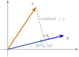
• The inner product \(x \cdot y\) directly measures how much \(y\) extends in the direction of \(x\)

  \[ \text{proj}_{x}(y) = \frac{x \cdot y}{x \cdot x} \, x \]

  • The scalar \(\tfrac{x \cdot y}{x \cdot x}\) is the signed length of \(y\)’s shadow along \(x\) (relative to \(\|x\|\)).
  • \(x \cdot y\) is large when \(y\) points strongly in the direction of \(x\), zero when \(x \perp y\)

Orthogonality

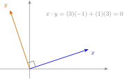
• When \(x \cdot y = 0\), the projection vanishes
• \(y\) has no component in the direction of \(x\). The vectors are perpendicular.

Linear Combinations

• A linear combination of vectors \(x^1, \ldots, x^n\) is a vector of the form \(\alpha_1 x^1 + \ldots + \alpha_n x^n\) for some \(\alpha_1, \ldots, \alpha_n \in \mathbb{R}\)
• Example 1: \(1 \times \begin{bmatrix} 1 & 2 & 3 \end{bmatrix}^\top + 2\times \begin{bmatrix} 4 & 5 & 6 \end{bmatrix}^\top = \begin{bmatrix} 1 & 2 & 3 \end{bmatrix}^\top + \begin{bmatrix} 8 & 10 & 12 \end{bmatrix}^\top = \begin{bmatrix} 9 & 12 & 15 \end{bmatrix}^\top\)
• Example 2: Can I construct \(y = \begin{bmatrix}2 & 1\end{bmatrix}^\top\) from \(x^1 = \begin{bmatrix} 1 & 2 \end{bmatrix}^{\top}\) and \(x^2 = \begin{bmatrix} -1 & 0 \end{bmatrix}^{\top}\)?
  • \(y = 0.5 x^1 - 1.5 x^2\)

• Show constructing a vector from unit vectors.
• Show the \(y\) and \(x_1\) and \(x^2\) in this exact example.

Linear Independence

• With \(k\) vectors \(x^1, \ldots, x^k\) in \(\mathbb{R}^n\): they are linearly independent if the only solution to \(\alpha_1 x^1 + \cdots \alpha_k x^k = \begin{bmatrix} 0 & \ldots & 0 \end{bmatrix}^\top\) is \(\alpha_1, \ldots, \alpha_k = 0\)
  • i.e., the only linear combination that yields the zero vector is the trivial one.
• Alternatively, you could find a counterexample by showing that a vector in the set can be written as a linear combination of the other vectors.

Linear Independence Example

• Pairwise comparisons are not enough. Example:
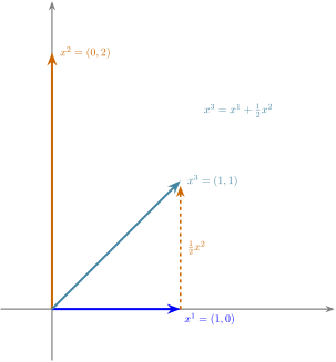
  • \(x^1 = \begin{bmatrix} 1 \\ 0 \end{bmatrix}, x^2 = \begin{bmatrix} 0 \\ 2 \end{bmatrix}, x^3 = \begin{bmatrix} 1 \\ 1 \end{bmatrix}\) then the \(\{x^1, x^2, x^3\}\) are never collinear pairwise
  • However, the set is not linearly independent since \(x^3 = x^1 + \frac{1}{2} x^2\)
  • Alternatively, note that \(1 \times x^1 + \frac{1}{2} \times x^2 + (-1) \times x^3 = \begin{bmatrix} 0 & 0 \end{bmatrix}^\top\), i.e. \(\alpha_1 = 1, \alpha_2 = \frac{1}{2}, \alpha_3 = -1\) is a non-trivial linear combination that yields the zero vector

Span

• Given a set of vectors, can you reach a particular point through some linear combination?
• Generalizes to \(\text{span}(x^1, \ldots, x^k) = \{y \in \mathbb{R}^n \,:\, y = \alpha_1 x^1 + \ldots + \alpha_k x^k\) for some \(\alpha_1, \ldots, \alpha_k \in \mathbb{R}\} \subseteq \mathbb{R}^n\)
• With \(k \leq n\) linearly independent vectors \(x^1, \ldots, x^k\) in \(\mathbb{R}^n\), the dimension of the span is \(k\).
  • In particular, with \(n\) vectors you can reach any point in \(\mathbb{R}^n\)
  • e.g., with 2 vectors in \(\mathbb{R}^3\) at most can reach a plane in \(\mathbb{R}^3\), but if vectors are collinear then they can only reach points along a line

Dimension of the Span

• Any collinearity has lower dimension
• e.g., If \(x^1\) and \(x^2\) are collinear, then the span is a line in \(\mathbb{R}^n\)
  • e.g., \(x^1 = \begin{bmatrix} 1 \\ 2 \\ 3 \end{bmatrix}, x^2 = \begin{bmatrix} 2 \\ 4 \\ 6 \end{bmatrix}\) then the span is \(\{\alpha x^1\,:\,\text{for all } \alpha \in \mathbb{R}\}\)
• Crucial for intuition on identification and independence of your data
  • e.g., if an observable in my data is a linear combination of other observables, then OLS cannot separately identify its effects

Matrices

Matrices

• \(A = \begin{bmatrix} A_{11} & \ldots & A_{1m} \\ \cdots & \ddots & \vdots \\ A_{n1} & \dots & A_{nm} \end{bmatrix} \in \mathbb{R}^{n \times m}\)
• Denote \(A_{ij}\) as the element in row \(i=1,\ldots,n\) and column \(j=1,\ldots,m\)

Matrix Transpose

• Definition: \((A^\top)_{ij} = A_{ji}\)
• Example: \(\begin{bmatrix}1 & 2 & 3 \\ 0 & -6 & 7 \end{bmatrix}^\top = \begin{bmatrix}1 & 0 \\ 2 & -6 \\ 3 & 7 \end{bmatrix}\)
• Note: \((A^\top)^\top = A\)

Matrices and Vectors

• Column vector: \(v \in \mathbb{R}^{n \times 1}\) and row vector: \(u \in \mathbb{R}^{1 \times n}\)
  • \(x = \begin{bmatrix} x_1 \\ x_2 \\ \vdots \\ x_n\end{bmatrix}\)
• Transpose: \(x^\top = \begin{bmatrix} x_1 & x_2 & \ldots & x_n\end{bmatrix}\)

Matrix Addition/Subtraction

• Definition: \((A + B)_{ij} = A_{ij} + B_{ij}\) (pointwise)
• Example: \(\begin{bmatrix} 1 & 3 \\ 1 & 0 \end{bmatrix} + \begin{bmatrix}0 & 0 \\ 7 & 5 \end{bmatrix} = \begin{bmatrix}1 & 3 \\ 8 & 5 \end{bmatrix}\)

Properties of Addition

• Commutativity: \(A + B = B + A\)
• Associativity: \((A + B) + C = A + (B + C)\)
• \((A + B)^\top = A^\top + B^\top\)

Matrix Multiplication

• For \(A \in \mathbb{R}^{n \times m}\) and \(B \in \mathbb{R}^{m \times p}\), the product \(C = AB \in \mathbb{R}^{n \times p}\)
  • Note inner dimensions, \(m\) and \(m\) must match or it doesn’t conform
• Calculation: \(C_{ik} = \sum_{j=1}^{m} A_{ij}B_{jk}\)

Matrix Multiplication Example

\[ \begin{bmatrix} a_{11} & a_{12} \\ a_{21} & a_{22} \end{bmatrix} \begin{bmatrix} b_{11} & b_{12} \\ b_{21} & b_{22} \end{bmatrix} = \begin{bmatrix} a_{11}b_{11} + a_{12}b_{21} & a_{11}b_{12} + a_{12}b_{22} \\ a_{21}b_{11}+a_{22}b_{21} & a_{21}b_{12}+a_{22}b_{22} \end{bmatrix} \]

Matrix Multiplication Properties

• \((AB)^\top = B^\top A^\top\)
• Associativity: \((AB)C = A(BC)\)
• Right distributivity: \((A+B)C = AC + BC\)
• Left distributivity: \(A(B+C) = AB + AC\)
• NOT commutative: \(AB \neq BA\) in general

Commutativity and Multiplication

• Scalar multiplication is commutative: \(\alpha A = A \alpha\)
• Matrix multiplication is not:
  • \(\begin{bmatrix}1 & 2 \\ 3 & 4 \end{bmatrix} \begin{bmatrix}0 & 1 \\ 0 & 0 \end{bmatrix} = \begin{bmatrix}0 & 1 \\ 0 & 3 \end{bmatrix}\)
  • \(\begin{bmatrix}0 & 1 \\ 0 & 0 \end{bmatrix} \begin{bmatrix}1 & 2 \\ 3 & 4 \end{bmatrix} = \begin{bmatrix}3 & 4 \\ 0 & 0 \end{bmatrix}\)
• Key Trick: be careful on whether operations are done from the left or right, then apply commutativity where appropriate

Matrix-Vector as Dot Products

• Sometimes algebra with matrix vector products are easier to construct with inner products

\[ \begin{bmatrix}1 & 2 \\ 3 & 4 \\ 5 & 6 \end{bmatrix} \begin{bmatrix}3 \\ -1 \end{bmatrix} = \begin{bmatrix} \begin{bmatrix}1 & 2 \end{bmatrix} \cdot \begin{bmatrix}3 & -1 \end{bmatrix} \\ \begin{bmatrix}3 & 4 \end{bmatrix} \cdot \begin{bmatrix}3 & -1 \end{bmatrix} \\ \begin{bmatrix}5 & 6 \end{bmatrix} \cdot \begin{bmatrix}3 & -1 \end{bmatrix} \end{bmatrix} = \begin{bmatrix} 1 \\ 5 \\ 9 \end{bmatrix} \]

• Many roles, but can also help with algebra
• \(2 x + 3 y = 10, 4 x - 2 y = 1\) becomes \(\begin{bmatrix}2 & 3\end{bmatrix} \cdot \begin{bmatrix}x \\ y\end{bmatrix} = 10\), etc.

Matrix-Vector as Linear Combinations

• Partition a matrix, \(A\), by its columns
  • \(\mathbf{a_i} \equiv \begin{bmatrix} a_{i1} & a_{i2} & \cdots & a_{in} \end{bmatrix}^\top \in \mathbb{R}^n\) as the \(i\)-th column of \(A\), so that \(A = \begin{bmatrix} \mathbf{a}_1 & \mathbf{a}_2 & \cdots & \mathbf{a}_m \end{bmatrix} \in \mathbb{R}^{n \times m}\)
• Then for any \(b = \begin{bmatrix} b_1 & b_2 & \cdots & b_m \end{bmatrix}^\top \in \mathbb{R}^m\)

\[ A b = b_1\mathbf{a}_1 + b_2\mathbf{a}_2 + \cdots + b_m\mathbf{a}_m \]

• i.e., a linear combination of the columns of \(A\), weighted by the entries of \(b\)

• For example, let the \(A\) matrix be a bunch of observations in a row, with observables in the columns (ML people call these “features”). e.g. gender and wealth.
• Then \(A b\) is constructing some set of outputs for each “observable” as a linear combination of the “features”.
• A linear regression, in this sense, \(A b = y\) is trying to find the best \(b\) which will try to match the observables. The \(b\) are the relative importance of each feature.
• If we had \(\mathbf{a}_1 = \mathbf{a}_2\) then could rearrange the linear combination so that many different \(b_1\) and \(b_2\) produce the same \(A b\). True also if \(b_1 \propto b_2\).

Matrix Inverse and Systems

Identity Matrix

• \(I = \begin{bmatrix} 1 & 0 & \cdots & 0 \\ 0 & 1 & \cdots & 0 \\ \vdots & \vdots & \ddots & \vdots \\ 0 & 0 & \cdots & 1 \end{bmatrix}\): ones on the diagonal, zeros elsewhere
• Property: \(I A = A\) for matrices or vectors
• Commutes: \(IA = AI = A\)

Matrix Inverse

• If \(A\) is square and \(F\) satisfies \(FA = I\), then \(F = A^{-1}\)
• \(A\) is invertible/nonsingular
• \(AA^{-1} = A^{-1}A = I\)
• Warning: \(A/B\) is meaningless (is it \(A^{-1}B\) or \(BA^{-1}\)?)

Inverse Properties

Diagonal matrix inverse

If \(D = \mathrm{diag}(d_1, \ldots, d_n)\) with all \(d_i \neq 0\): \[D^{-1} = \mathrm{diag}\!\left(\tfrac{1}{d_1}, \ldots, \tfrac{1}{d_n}\right)\]

Exercise: \((AB)^{-1} = B^{-1}A^{-1}\)

Show that \(B^{-1}A^{-1}\) is the inverse of \(AB\).

Worked solution

Trivial Inverses (and Failures)

• \(A = \begin{bmatrix} a \end{bmatrix}\) (i.e., a scalar), then \(A^{-1} = \begin{bmatrix} \frac{1}{a} \end{bmatrix}\)
• \(A = \begin{bmatrix} a & 0 \\ 0 & b \end{bmatrix}\), then \(A^{-1} = \begin{bmatrix} \frac{1}{a} & 0 \\ 0 & \frac{1}{b} \end{bmatrix}\)
  • Unless \(a = 0\) or \(b = 0\) in which case \(A\) is not invertible
• If \(A = \begin{bmatrix} 1 & 2 \\ 3 & 6 \end{bmatrix}\) then \(A\) is not invertible
  • i.e., second column is \(2 \times\) the first

Systems of Equations

• Must be square, \(n \times n\)!
• System: \(Ax = b\) where \(A \in \mathbb{R}^{n \times n}\), \(x \in \mathbb{R}^{n \times 1}\), \(b \in \mathbb{R}^{n \times 1}\)
• Unique solution if \(A\) is invertible:
  • Left multiply by \(A^{-1}\) to get \(A^{-1}Ax = A^{-1}b\)
  • Then use \(A^{-1}A = I\)
  • And then \(Ix = x\) to yield: \(x = A^{-1}b\)

System Example

\[ \{2x + 3y = 2, \quad x - 2y = -1\} \Rightarrow \begin{bmatrix}2 & 3 \\ 1 & -2 \end{bmatrix} \begin{bmatrix}x \\ y \end{bmatrix} = \begin{bmatrix} 2 \\ -1 \end{bmatrix} \]

\[ \Rightarrow \begin{bmatrix}x \\ y \end{bmatrix} = \begin{bmatrix}2 & 3 \\ 1 & -2 \end{bmatrix}^{-1} \begin{bmatrix} 2 \\ -1 \end{bmatrix} \]

Vector Selection

• Extract second element from \(x = \begin{bmatrix}x_1 & x_2 & x_3 \end{bmatrix}^\top\):
• \(x_2 = \begin{bmatrix} 0 & 1 & 0\end{bmatrix} \begin{bmatrix} x_1 \\ x_2 \\ x_3 \end{bmatrix}\)
• Use vector with single \(1\) and \(0\)s elsewhere

PhD MaterialPhD

Additional Topics

Topics covered:

• Column space, rank, and identification
• Projection onto the column space
• The structure of \(X'X\): symmetry, eigendecomposition, and definiteness
• Quadratic forms, Cholesky decomposition

Matrices as DataPhD

Matrices as Data: Rows and Columns

The key mental model for econometrics: \(X \in \mathbb{R}^{n \times k}\) is a data matrix.

• Row \(i\): the \(k\) attributes (regressors) observed for unit \(i\)
• Column \(j\): the \(n\) observations of the \(j\)-th variable

The product \(X\beta\) gives a vector in \(\mathbb{R}^n\): the \(i\)-th entry is a weighted combination of unit \(i\)’s attributes: \[ (X\beta)_i = x_i'\beta = \beta_1 x_{i1} + \cdots + \beta_k x_{ik} \]

A central question: do the columns of \(X\) contain redundant information? If so, many different \(\beta\) vectors produce the same \(X\beta\) — the weight vector cannot be uniquely recovered from the product alone.

Example: The Iris Data Matrix

Predict sepal length from sepal width and petal length (\(n = 150\) flowers, \(k = 3\) columns including intercept):

	Int	SW	PL	\(y\)
Setosa 1	1	3.5	1.4	5.1
Setosa 2	1	3.0	1.4	4.9
Versicol. 3	1	3.2	4.7	7.0
Versicol. 4	1	3.2	4.5	6.4
Virginica 5	1	3.3	6.0	6.3

\[ X = \begin{pmatrix} 1 & 3.5 & 1.4 \\ 1 & 3.0 & 1.4 \\ 1 & 3.2 & 4.7 \\ 1 & 3.2 & 4.5 \\ 1 & 3.3 & 6.0 \end{pmatrix} \quad y = \begin{pmatrix} 5.1 \\ 4.9 \\ 7.0 \\ 6.4 \\ 6.3 \end{pmatrix} \]

\(X\beta = \beta_1\mathbf{1} + \beta_2 x_{(\text{sw})} + \beta_3 x_{(\text{pl})}\): each row gives one predicted sepal length.

The Column Space

For a data matrix \(X\) (\(n \times k\)), the column space is the set of all outcome vectors the model can reproduce exactly: \[ \text{col}(X) = \{X\beta : \beta \in \mathbb{R}^k\} = \text{span of the columns of } X \]

Each column of \(X\) is one regressor across all \(n\) observations. Finding which linear combination of these columns lies closest to a given \(y\) is the projection problem we address later.

Rank

The rank of \(X\) is the number of linearly independent columns — the number of regressors that genuinely contribute new information: \[ \text{rank}(X) = \dim(\text{col}(X)) \leq \min(n, k) \]

Full Rank: Independent Regressors

\[ X = \begin{pmatrix} 1 & 10 \\ 1 & 15 \\ 1 & 20 \end{pmatrix} \qquad \text{Columns: intercept } x_{(1)} \text{ and income } x_{(2)}\text{, three observations} \]

Can we write \(x_{(2)} = \alpha \, x_{(1)}\)? We need \((10,15,20) = \alpha(1,1,1)\), which requires \(\alpha = 10, 15, 20\) simultaneously — impossible. The columns are linearly independent, \(\text{rank}(X) = 2\), and \(\beta_1\) and \(\beta_2\) can be separately identified from \(X\beta\).

Rank Deficiency: Perfect Multicollinearity

\[ X = \begin{pmatrix} 1 & 10 & 20 \\ 1 & 15 & 30 \\ 1 & 20 & 40 \end{pmatrix} \qquad \text{Columns: intercept, income, } 2\times\text{income} \]

Column 3 \(= 2\times\) column 2: the third regressor is redundant. Consequently:

• For any \(\beta\), the vector \(\tilde{\beta} = \beta + \gamma\begin{pmatrix} 0 \\ 1 \\ -1/2 \end{pmatrix}\) gives identical predictions \(X\beta = X\tilde{\beta}\) for every \(\gamma\)
• \(\text{rank}(X) = 2 < 3\): only two of the three columns are linearly independent, so \(X'X\) is singular
• The individual effects of income and twice-income cannot be separately identified

ProjectionPhD

The Projection Problem

Setup

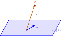
You have a vector \(y \in \mathbb{R}^n\) and a subspace \(S = \text{col}(X)\) — the span of the columns of an \(n \times k\) matrix \(X\).

Goal: Find the best linear approximation of \(y\) from the columns of \(X\) — the vector \(\hat{y} \in S\) that is closest to \(y\).

The Key Geometric Insight

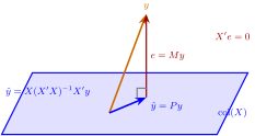
The closest point \(\hat{y}\) in \(\text{col}(X)\) to \(y\) is the one where the residual \(e = y - \hat{y}\) is perpendicular to the subspace.

Orthogonality condition

\(e\) must be orthogonal to every vector in \(\text{col}(X)\): \[ X'e = 0 \] Each column of \(X\) must be orthogonal to the residual.

Deriving the Projection Matrix

Since \(\hat{y} \in \text{col}(X)\), write \(\hat{y} = Xb\) for some \(b \in \mathbb{R}^k\). The residual is \(e = y - Xb\).

Applying \(X'e = 0\): \[ X'(y - Xb) = 0 \implies X'Xb = X'y \quad \text{(orthogonality conditions)} \]

If \(X\) has full column rank, \(X'X\) is invertible: \[ b = (X'X)^{-1}X'y \implies \hat{y} = Xb = X(X'X)^{-1}X'y \]

The projection matrix

\[ P = X(X'X)^{-1}X', \qquad \hat{y} = Py \]

The Projection: Geometric Summary

Properties of the Projection Matrix

Idempotent: \(P^2 = P\)

\[ P^2 = X(X'X)^{-1}\underbrace{X'X(X'X)^{-1}}_{I}X' = P \] Projecting twice is the same as projecting once.

Symmetric: \(P' = P\)

\[ P' = (X(X'X)^{-1}X')' = X((X'X)')^{-1}X' = X(X'X)^{-1}X' = P \]

The Annihilator Matrix \(M = I - P\)

Definition

\(M = I - P\) produces the residual: \(e = y - Py = My\).

\(M\) inherits the same properties: idempotent (\(M^2 = M\)) and symmetric (\(M' = M\)).

Key property: \(MX = 0\)

\[ MX = (I - P)X = X - X(X'X)^{-1}X'X = X - X = 0 \] \(M\) annihilates anything in \(\text{col}(X)\) and keeps only the perpendicular part.

Rank and degrees of freedom

\(\text{rank}(P) = k\), \(\;\text{rank}(M) = n - k\), \(\;\text{tr}(M) = n - k\).

This is why \(n - k\) is called degrees of freedom: it is the dimension of the space the residuals live in.

Practice: The Projection and Annihilator Matrices

Practice: Properties of \(P\) and \(M\)

Let \(P = X(X'X)^{-1}X'\) and \(M = I - P\), with \(X\) of full column rank.

1. Show \(P\) is idempotent (\(P^2 = P\)) and symmetric (\(P' = P\)).
2. Show \(MX = 0\), and interpret it geometrically.
3. Show \(PM = 0\), and conclude the fitted values \(Py\) and residuals \(My\) are orthogonal.

Worked solution

When Is the Projection Formula Valid?

The expression \(P = X(X'X)^{-1}X'\) requires \((X'X)^{-1}\) to exist. The equivalent conditions are:

Equivalent conditions for \((X'X)^{-1}\) to exist

• The columns of \(X\) are linearly independent (no perfect multicollinearity)
• \(\text{rank}(X) = k\) (full column rank)
• Each regressor carries information not already captured by the others

When any of these fail, \(X'X\) is singular, the formula breaks down, and the coefficient vector \(b\) with \(\hat{y} = Xb\) is not unique — many \(b\)’s yield the same closest approximation of \(y\).

The Structure of \(X'X\)PhD

\(X'X\): From Projection to Deeper Structure

The projection \(\hat{y} = X(X'X)^{-1}X'y\) depends on \(X'X\) being invertible. But \(X'X\) has richer structure worth understanding on its own terms: it is always symmetric, and its eigenvalues and eigenvectors encode how much independent information the columns of \(X\) carry.

Symmetric Matrices

Definition

A square matrix \(A\) is symmetric if \(A = A'\), i.e., \(a_{ij} = a_{ji}\) for all \(i, j\).

The \((i,j)\) entry of \(X'X\) is the inner product \(x_{(i)} \cdot x_{(j)}\) of regressor columns \(i\) and \(j\) — and inner products are symmetric. So \(X'X\) is always symmetric:

\[ (X'X)' = X'(X')' = X'X \quad \checkmark \]

Eigenvectors

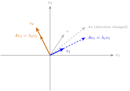
For most vectors \(v\), \(Av\) is a vector not proportional to \(v\). But some vectors are special: \(Av\) is just a scalar multiple of \(v\).

Definition

A nonzero vector \(v\) is an eigenvector of \(A\) if \[ Av = \lambda v \] for some scalar \(\lambda\). The scalar \(\lambda\) is the corresponding eigenvalue.

\(\lambda > 1\): \(v\) stretched. \(\quad\) \(0 < \lambda < 1\): \(v\) compressed. \(\quad\) \(\lambda < 0\): \(v\) negated and scaled.

Verifying Eigenvectors

Example: \(A = \begin{pmatrix} 3 & 1 \\ 1 & 2 \end{pmatrix}\)

Claim: \(v_1 = \begin{pmatrix} 1 \\ 0.62 \end{pmatrix}\) is an eigenvector with \(\lambda_1 \approx 3.62\).

Check: \(Av_1 = \begin{pmatrix} 3 & 1 \\ 1 & 2 \end{pmatrix}\begin{pmatrix} 1 \\ 0.62 \end{pmatrix} = \begin{pmatrix} 3.62 \\ 2.24 \end{pmatrix} \approx 3.62 \begin{pmatrix} 1 \\ 0.62 \end{pmatrix}\) \(\checkmark\)

Second eigenvector

Claim: \(v_2 = \begin{pmatrix} 1 \\ -1.62 \end{pmatrix}\) is an eigenvector with \(\lambda_2 \approx 1.38\).

Check: \(Av_2 = \begin{pmatrix} 3 & 1 \\ 1 & 2 \end{pmatrix}\begin{pmatrix} 1 \\ -1.62 \end{pmatrix} = \begin{pmatrix} 1.38 \\ -2.24 \end{pmatrix} \approx 1.38 \begin{pmatrix} 1 \\ -1.62 \end{pmatrix}\) \(\checkmark\)

Diagonalization

Stack all eigenvector equations \(Av_i = \lambda_i v_i\) into one matrix equation:

\[ A \underbrace{\begin{pmatrix} v_1 & \cdots & v_n \end{pmatrix}}_{P} = \underbrace{\begin{pmatrix} v_1 & \cdots & v_n \end{pmatrix}}_{P} \underbrace{\begin{pmatrix} \lambda_1 & & \\ & \ddots & \\ & & \lambda_n \end{pmatrix}}_{D} \]

So \(AP = PD\), which gives:

Eigendecomposition

\[A = PDP^{-1}\] where \(P\) has eigenvectors as columns and \(D = \text{diag}(\lambda_1, \ldots, \lambda_n)\).

For symmetric \(A\): \(P\) is orthogonal (\(P^{-1} = P'\)), so \(A = PDP'\).

What Diagonalization Tells You

Key insight

A matrix transformation is completely pinned down by its eigenvalues and eigenvectors.

If you know the eigenvectors (the special vectors \(A\) scales) and the eigenvalues (the scale factors), you can reconstruct \(A\) entirely.

Our running example

\[ \underbrace{\begin{pmatrix} 3 & 1 \\ 1 & 2 \end{pmatrix}}_{A} = \underbrace{\begin{pmatrix} 1 & 1 \\ 0.62 & -1.62 \end{pmatrix}}_{P} \underbrace{\begin{pmatrix} 3.62 & 0 \\ 0 & 1.38 \end{pmatrix}}_{D} \underbrace{\begin{pmatrix} 1 & 1 \\ 0.62 & -1.62 \end{pmatrix}^{-1}}_{P^{-1}} \]

Practice: Properties of Symmetric Matrices

Eigenvectors with distinct eigenvalues are orthogonal

Let \(A = A'\), \(Av_1 = \lambda_1 v_1\), \(Av_2 = \lambda_2 v_2\) with \(\lambda_1 \neq \lambda_2\).

Show \(v_1' v_2 = 0\).

Orthonormal eigenvectors give \(P^{-1} = P'\)

If \(P\) has orthonormal columns (\(v_i' v_j = 0\) for \(i \neq j\), \(v_i'v_i = 1\)), show \(P'P = I\) and conclude \(P^{-1} = P'\).

Every PD matrix factors as \(K'K\)

Let \(A = PDP'\) with all \(\lambda_i > 0\). Define \(D^{1/2} = \mathrm{diag}(\sqrt{\lambda_1}, \ldots, \sqrt{\lambda_n})\) and set \(K = D^{1/2}P'\).

Show \(K'K = A\) and conclude every PD matrix can be written as \(K'K\) for invertible \(K\).

Solution: orthogonality Solution: inverse = transpose Solution: PD factorization

Eigenvectors: Geometric Picture (Optional)

Eigenvectors of \(A = \begin{pmatrix} 3 & 1 \\ 1 & 2 \end{pmatrix}\) (Optional)

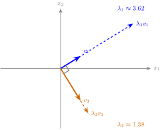
For this symmetric matrix, \(v_1 \perp v_2\): \(v_1' v_2 = (1)(1) + (0.62)(-1.62) \approx 0\). (See Practice 1 above.)

Quadratic Forms and DefinitenessPhD

The Quadratic Form

Definition

Given a symmetric \(n \times n\) matrix \(A\), the quadratic form is the function \[ q(x) = x'Ax \] It takes a vector \(x \in \mathbb{R}^n\) and returns a scalar.

Example: \(A = \begin{pmatrix} 3 & 1 \\ 1 & 2 \end{pmatrix}\)

\[ q(x) = \begin{pmatrix} x_1 & x_2 \end{pmatrix}\begin{pmatrix} 3 & 1 \\ 1 & 2 \end{pmatrix}\begin{pmatrix} x_1 \\ x_2 \end{pmatrix} = 3x_1^2 + 2x_1 x_2 + 2x_2^2 \]

Positive Definite Matrices

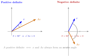
Positive definiteness is the matrix analog of a positive real number: just as \(a > 0\) means \(ax\) never “opposes” \(x\), a PD matrix never produces a negative quadratic form.

Definition

A symmetric matrix \(A\) is positive definite (PD) if \(x'Ax > 0\) for all \(x \neq 0\).

Equivalent characterization via eigenvalues

\(A\) is positive definite \(\;\Longleftrightarrow\;\) all eigenvalues are strictly positive: \(\lambda_i > 0\) for all \(i\).

Since \(\det(A) = \prod_i \lambda_i\), every PD matrix is invertible.

Positive semidefinite (PSD)

\(A\) is positive semidefinite if \(x'Ax \geq 0\) for all \(x\) — equivalently, all \(\lambda_i \geq 0\).

\(A\) is indefinite if it has both positive and negative eigenvalues.

Quadratic Forms and Eigenvalues

Using the spectral decomposition \(A = PDP'\), let \(z = P'x\) (coordinates along eigenvector directions):

Quadratic form in eigenvector coordinates

\[ x'Ax = x'PDP'x = z'Dz = \lambda_1 z_1^2 + \lambda_2 z_2^2 + \cdots + \lambda_n z_n^2 \]

Why the eigenvalue condition works

The quadratic form is a weighted sum of squares with weights \(\lambda_i\). It is positive for every \(z \neq 0\) if and only if every weight is positive — exactly the PD condition.

Practice: Quadratic Forms in Eigenvector Coordinates

Practice: Diagonalizing the quadratic form

Let \(A = PDP'\) be symmetric (\(P\) orthogonal, \(D = \mathrm{diag}(\lambda_1, \ldots, \lambda_n)\)), and set \(z = P'x\).

1. Show \(x'Ax = \sum_{i=1}^n \lambda_i z_i^2\).
2. Use this to prove \(A\) is positive definite if and only if every \(\lambda_i > 0\).

Worked solution

\(X'X\): Definiteness and Rank

For any matrix \(X\), \(X'X\) is positive semidefinite: \(\;c'X'Xc = \|Xc\|^2 \geq 0\).

Result

\(X'X\) is positive definite \(\;\Longleftrightarrow\;\) \(X\) has full column rank \(\;\Longleftrightarrow\;\) \(X'X\) is invertible.

\(X'X\): Full Rank vs. Rank Deficient

Full column rank: \(X'X\) is positive definite

\[X = \begin{pmatrix} 1 & 0 \\ 0 & 1 \\ 1 & 1 \end{pmatrix}\]

For any \(c = (c_1, c_2)' \neq 0\): \(\;c'X'Xc = \|Xc\|^2 = c_1^2 + c_2^2 + (c_1+c_2)^2 > 0\) \(\checkmark\)

Rank deficient: \(X'X\) is only positive semidefinite

\[X = \begin{pmatrix} 1 & 2 \\ 2 & 4 \\ 3 & 6 \end{pmatrix} \quad (\text{col}_2 = 2\cdot\text{col}_1)\]

Take \(c = (2, -1)'\): \(\;Xc = 0\), so \(c'X'Xc = \|Xc\|^2 = 0\) with \(c \neq 0\). \(X'X\) is not PD. ✗

Practice: \(X'X\) Definiteness

Prove the result: \(X'X\) is PD \(\iff\) \(X\) has full column rank

Key identity: \(c'X'Xc = \|Xc\|^2\).

1. (\(\Rightarrow\)) If \(X\) has full column rank, show \(c'X'Xc > 0\) for all \(c \neq 0\).
2. (\(\Leftarrow\)) If \(X\) is rank deficient, find a specific \(c \neq 0\) with \(c'X'Xc = 0\).
3. Invertibility: Why does this, combined with the result on the PD definition slide, imply \(X'X\) is invertible if and only if \(X\) has full column rank?

Worked solution

Cholesky Decomposition

Cholesky factorization

Every positive definite matrix \(\Sigma\) can be written uniquely as \[ \Sigma = LL' \] where \(L\) is lower triangular with strictly positive diagonal entries.

Example

\[ \begin{pmatrix} 4 & 2 \\ 2 & 3 \end{pmatrix} = \underbrace{\begin{pmatrix} 2 & 0 \\ 1 & \sqrt{2} \end{pmatrix}}_{L} \underbrace{\begin{pmatrix} 2 & 1 \\ 0 & \sqrt{2} \end{pmatrix}}_{L'} \quad\checkmark \]

Cholesky in Econometrics

Core applications

Sampling correlated normals. To draw \(\varepsilon \sim \mathcal{N}(0, \Sigma)\): factor \(\Sigma = LL'\), draw \(z \sim \mathcal{N}(0, I)\), set \(\varepsilon = Lz\). The covariance of \(Lz\) is \(L \cdot I \cdot L' = \Sigma\). \(\checkmark\)

Solving symmetric linear systems stably. Rather than inverting a positive definite matrix \(A\) directly, decompose \(A = LL'\) and solve two triangular systems \(Lv = b\) then \(L'x = v\) to find \(x = A^{-1}b\). Triangular solves are far more numerically stable than direct inversion for ill-conditioned matrices.

Positive Definiteness: Geometric Picture (Optional)

For symmetric \(A\), positive definiteness has a clean vector interpretation: \(x'Ax > 0\) means \(x \cdot Ax > 0\), i.e., \(x\) and \(Ax\) always point into the same half-space — they form an acute angle.