Optimization
UBC Economics Math Camps
Lecture Videos
Basic calculus
Definitions
- A function is a mapping connecting any element in a domain \(D\) to a codomain \(C\)
- Formally represented as
\[ f: D \mapsto C \]
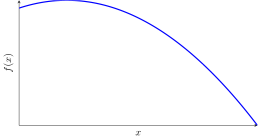
Simple example
- \(f(x) = - (x - 1)^2\)
Another example
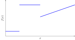
- Piece-wise definition:
\[ f(x) = \begin{cases} -1 &\text{, if }x < 2\\ 10&\text{, if } 2 \leq x \leq 5\\ x&\text{, if } x > 5 \end{cases} \]
Continuity
- Continuous functions do not feature “jumps”.
- The first example was a continuous function.
- The second example was a discontinuous function.
- A function is continuous at \(x \in D\) if
\[ \lim_{\tilde{x} \to x} f(\tilde{x}) = f(x) \]
The derivative as rise over run
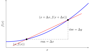
- The slope of the line through two points on the graph of \(f\) is
\[ \frac{\text{rise}}{\text{run}} = \frac{\Delta y}{\Delta x} = \frac{f(x + \Delta x) - f(x)}{\Delta x}. \]
- This is the slope of the secant line joining \((x, f(x))\) and \((x + \Delta x, f(x + \Delta x))\).
- As \(\Delta x \to 0\), the secant line rotates toward the tangent line at \(x\) — its slope is the derivative \(f'(x)\).
Derivatives
Single variable case:
- Rate of growth of \(f\): \(\frac{f(x + \varepsilon ) - f(x)}{\varepsilon }\).
- Derivative definition \(f'(x) = \lim_{\varepsilon \rightarrow 0, \varepsilon \neq 0} \frac{f(x + \varepsilon ) - f(x)}{\varepsilon }\).
- Local rate of growth of function.
- Second derivative: \(f''(x) = \lim_{\varepsilon \rightarrow 0, \varepsilon \neq 0} \frac{f'(x + \varepsilon ) - f'(x)}{\varepsilon } = (f')'(x)\)
Derivatives
Multiple variable case:
Rate of growth of \(f\) when single argument \(x_i\) changes: \(\frac{ f (x_1,\ldots , x_i + \varepsilon ,\ldots ,x_n) - f(x) }{\varepsilon }\)
Partial derivative: \(\frac{\partial f(x)}{\partial x_i} = \lim_{\varepsilon \rightarrow 0, \varepsilon \neq 0} \frac{ f (x_1,\ldots , x_i + \varepsilon ,\ldots ,x_n) - f(x) }{\varepsilon }\)
The gradient is a vector whose entries are all partial derivatives: \(\nabla f (x)= \left[ \frac{\partial f(x)}{\partial x_i} \right]_i\)
Example: if \(f(x_1, x_2) = x_1^2 + 3x_1 x_2\) then
\[ \nabla f (x) = \begin{bmatrix} 2x_1 + 3x_2 \\ 3 x_1 \end{bmatrix} \]
Rules of differentiation
Let \(f\) and \(g\) be differentiable functions and let \(c\) and \(n\) be constants.
| Rule | Function | Derivative |
|---|---|---|
| Constant | \(c\) | \(0\) |
| Constant multiple | \(c\,f(x)\) | \(c\,f'(x)\) |
| Sum / difference | \(f(x) \pm g(x)\) | \(f'(x) \pm g'(x)\) |
| Product | \(f(x)\,g(x)\) | \(f'(x)\,g(x) + f(x)\,g'(x)\) |
| Quotient | \(\dfrac{f(x)}{g(x)}\) | \(\dfrac{f'(x)\,g(x) - f(x)\,g'(x)}{\left[g(x)\right]^2}\) |
| Chain | \(f\bigl(g(x)\bigr)\) | \(f'\bigl(g(x)\bigr)\,g'(x)\) |
| Power | \(\left[f(x)\right]^n\) | \(n\left[f(x)\right]^{n-1} f'(x)\) |
| Inverse function | \(f^{-1}(x)\) | \(\dfrac{1}{f'\bigl(f^{-1}(x)\bigr)}\) |
The quotient rule requires \(g(x) \neq 0\), and the inverse function rule requires \(f'\bigl(f^{-1}(x)\bigr) \neq 0\).
The chain rule
- The chain rule does most of the work in practice: every composite function goes through it.
- Differentiate from the outside in — take the derivative of the outer function, leave the inside untouched, then multiply by the derivative of the inside:
\[ \frac{d}{dx} f\bigl(g(x)\bigr) = \underbrace{f'\bigl(g(x)\bigr)}_{\text{outer, inside kept}} \times \underbrace{g'(x)}_{\text{inner}}. \]
- Equivalently, writing \(y = f(u)\) with \(u = g(x)\):
\[ \frac{dy}{dx} = \frac{dy}{du}\,\frac{du}{dx}. \]
Derivatives of common functions
The third column is the chain rule applied to each row, for a differentiable inner function \(g\).
| \(f(x)\) | \(f'(x)\) | \(\dfrac{d}{dx} f\bigl(g(x)\bigr)\) |
|---|---|---|
| \(c\) | \(0\) | \(0\) |
| \(x^n\) | \(n x^{n-1}\) | \(n \left[g(x)\right]^{n-1} g'(x)\) |
| \(\sqrt{x}\) | \(\dfrac{1}{2\sqrt{x}}\) | \(\dfrac{g'(x)}{2\sqrt{g(x)}}\) |
| \(\dfrac{1}{x}\) | \(-\dfrac{1}{x^2}\) | \(-\dfrac{g'(x)}{\left[g(x)\right]^2}\) |
| \(e^x\) | \(e^x\) | \(e^{g(x)}\, g'(x)\) |
| \(a^x\) | \(a^x \ln a\) | \(a^{g(x)} \ln(a)\, g'(x)\) |
| \(\ln x\) | \(\dfrac{1}{x}\) | \(\dfrac{g'(x)}{g(x)}\) |
| \(\log_a x\) | \(\dfrac{1}{x \ln a}\) | \(\dfrac{g'(x)}{g(x) \ln a}\) |
| \(\sin x\) | \(\cos x\) | \(\cos\bigl(g(x)\bigr) g'(x)\) |
| \(\cos x\) | \(-\sin x\) | \(-\sin\bigl(g(x)\bigr) g'(x)\) |
Domains: \(\sqrt{x}\) and \(\ln x\) require \(x > 0\); \(a^x\) and \(\log_a x\) require \(a > 0\) with \(a \neq 1\).
As is standard in economics, the rest of these slides write \(\log\) for the natural logarithm, so \(\log x \equiv \ln x\).
Applying the rules
Chain rule. For \(f(x) = 3(x+10)^3 + 20x\), the outer function is a cube and the inner function is \(x + 10\):
\[ f'(x) = 3 \cdot 3(x+10)^2 \cdot 1 + 20 = 9(x+10)^2 + 20. \]
Chain and quotient rules together. For \(f(x) = \log\!\left( \dfrac{x^2}{1+x} \right)\) with \(x > 0\), the log takes \(g(x) = \dfrac{x^2}{1+x}\), so \(f'(x) = g'(x)/g(x)\). The quotient rule gives
\[ g'(x) = \frac{2x(1+x) - x^2}{(1+x)^2} = \frac{x^2 + 2x}{(1+x)^2}, \qquad\text{so}\qquad f'(x) = \frac{x^2+2x}{(1+x)^2} \cdot \frac{1+x}{x^2} = \frac{x+2}{x(1+x)}. \]
Since logs turn quotients into differences, \(\log\!\left(\frac{x^2}{1+x}\right) = 2\log x - \log(1+x)\) is often the faster route to the same answer.
The same rules apply to partial derivatives
To compute \(\frac{\partial f(x)}{\partial x_i}\), treat every other variable as a constant and apply the single-variable rules above.
Example: the Cobb-Douglas utility \(u(x,y) = x^a y^b\) used later in this deck.
\[ \frac{\partial u}{\partial x} = a x^{a-1} y^{b}, \qquad \frac{\partial u}{\partial y} = b x^{a} y^{b-1}. \]
Holding \(y\) fixed, \(y^b\) is only a multiplicative constant, so the power rule in \(x\) does all the work — and symmetrically for \(y\).
Concavity
Definition
A function of \(n\) real numbers \(f(x)\) is concave if, for all \(x,x'\) and \(\alpha \in [0,1]\)
\[ \alpha f(x) + (1 - \alpha ) f(x') \leq f( \alpha x + (1 - \alpha )x'). \]
A function of \(n\) real numbers \(f(x)\) is convex if, for all \(x,x'\) and \(\alpha \in [0,1]\)
\[ \alpha f(x) + (1 - \alpha ) f(x') \geq f( \alpha x + (1 - \alpha )x'). \]
Definition – Strict version
A function of \(n\) real numbers \(f(x)\) is strictly concave if, for all \(x,x'\) and \(\alpha \in ( 0,1 )\)
\[ \alpha f(x) + (1 - \alpha ) f(x') < f( \alpha x + (1 - \alpha )x'). \]
A function of \(n\) real numbers \(f(x)\) is strictly convex if, for all \(x,x'\) and \(\alpha \in ( 0,1 )\)
\[ \alpha f(x) + (1 - \alpha ) f(x') > f( \alpha x + (1 - \alpha )x'). \]
Derivative characterization
Concavity is easier to check if the second derivative exists.
Single variable
\(f\) is concave if, and only if, \(f''(x) \mathbf{\leq} 0\) for all values \(x\).
- In other words: a concave function’s derivative must be decreasing.
\(f\) is convex if, and only if, \(f''(x) \mathbf{\geq} 0\) for all values \(x\).
Examples:
- \(f(x) = 0\) is concave since \(f'(x) = f''(x)=0\).
- \(f(x) = \log(x)\) is concave: \(f'(x) = \frac{1}{x}\) and \(f''(x) = -\frac{1}{x^2}<0\) (assume \(x>0\))
Derivative characterization
Single variable – Strict version
\(f\) is strictly concave if \(f''(x) \mathbf{<} 0\) for all values \(x\).
- In other words: a strictly concave function’s derivative must be strictly decreasing.
- \(f\) is still concave if \(f''(x) = 0\) for a single point.
\(f\) is strictly convex if \(f''(x) \mathbf{>} 0\) for all values \(x\).
Examples:
- \(f(x) = 0\) is concave, but not strictly so, since \(f'(x) = f''(x)=0\).
- \(f(x) = \log(x)\) is strictly concave since \(f''(x) = -\frac{1}{x^2}<0\) (restricting \(x>0\))
Derivative characterization
Multiple variables
A function of \(n\) variables has \(n^2\) possible second derivatives: \(\frac{\partial^2 f(x)}{\partial x_i\partial x_j} = \frac{\partial \left( \frac{\partial f(x)}{\partial x_i} \right) }{\partial x_j}\)
Hessian matrix collects them: \(H(x) = \left[ \frac{\partial^2 f(x)}{\partial x_i\partial x_j} \right]_{i,j}\)
A function \(f\) is concave if, and only if, \(H(x)\) is negative semi-definite for all values \(x\)
If \(H(\cdot )\) is negative definite then \(f\) is strictly concave.
Unconstrained optimization
Maximization and concavity
- \(x^*\) is a global maximizer (and \(f(x^*)\) a global maximum) of \(f\) if \(f(x^*) \geq f(x)\) for all \(x\)
- \(x^*\) is a global minimizer of \(f\) (and \(f(x^*)\) a global minimum) if \(f(x^*) \leq f(x)\) for all \(x\)
First order condition
Single variable
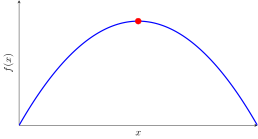
If \(x^*\) is a global maximizer or a global minimizer of \(f\), it must satisfy:
\[ f'(x^*) =0. \]
The zero-derivative condition is referred to as the first order condition (FOC).
The above statement means the FOC is necessary for optimality.
Second order condition
Single variable
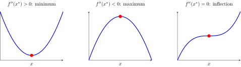
At a critical point where \(f'(x^*) = 0\), the sign of the second derivative tells us which kind of optimum we have:
- \(f''(x^*) < 0\): \(x^*\) is a local maximizer — \(f\) is strictly concave near \(x^*\).
- \(f''(x^*) > 0\): \(x^*\) is a local minimizer — \(f\) is strictly convex near \(x^*\).
- \(f''(x^*) = 0\): inconclusive — could be a maximizer, a minimizer, or an inflection point.
This is the local, calculus-based counterpart of the strict concavity/convexity definitions from the Concavity section.
First order condition
Multiple variables
If \(x^*\) is a global maximizer of \(f\), it must satisfy the following first-order condition
\[ \nabla f(x^*) = [0 \ldots 0]^T. \]
First order condition
How to find maxima of a function?
If the following are satisfied:
- \(\nabla f(x^*) = [0 \ldots 0]^T\) (FOC),
- \(f\) is concave (second order condition – SOC)
then \(f(x^*)\) is a global maximum of \(f\).
This means that, under concavity, the FOC is sufficient for maximization.
The same result holds if we substitute concave with convex and maximum with minimum.
Uniqueness
- If \(f\) is strictly concave, it has at most one maximizer.
- FOC is still necessary: any maximum must satisfy it.
- FOC is still sufficient: if a point satisfies FOC, it is the maximum.
Practice: A Single-Peaked Function
Practice: A single-peaked function
Find the global maximum of
\[ f(x) = -3x^2 + 12x - 5. \]
Verify that the FOC is sufficient here.
Practice: A Multi-Peaked Function
Practice: A multi-peaked function
Find all critical points of
\[ f(x) = -x^4 + 8x^2. \]
Classify each one using the second order condition, and determine the global maximum.
Failure of second order condition
- So it is easy to find maxima of concave functions.
- What about convex functions? They may not have a maximum!
- Example: \(f(x) = x^2\) which has \(f''(x) = 2\).
- It grows without bound as \(x\) grows.
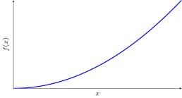
- The same occurs for minimizing concave functions.
Optimization with equality constraints
Example: Utility maximization
Consider a household whose utility is defined over consumption of two goods, \(x\) and \(y\):
\[ u(x,y)=x^a y^b. \]
Prices are \(p_x\) and \(p_y\); income is \(m\). Find the utility-maximizing demands.
Problem setup
\[ \begin{aligned} \max_{x,y} &\quad x^a y^b \\ \text{subject to} &\quad p_x x + p_y y = m. \end{aligned} \]
Example: Utility maximization
Lagrangian
\[ \mathcal{L}(x,y,\lambda) = x^a y^b + \lambda [m - p_x x - p_y y]. \]
Example continued
The first-order conditions with respect to \((x,y)\) are:
\[ \begin{aligned} \frac{\partial \mathcal{L}}{\partial x} &= a x^{a-1} y^b - \lambda p_x = 0, \\ \frac{\partial \mathcal{L}}{\partial y} &= x^a b y^{b-1} - \lambda p_y = 0. \end{aligned} \]
Example continued
With the budget constraint,
\[ m - p_x x - p_y y = 0, \]
we obtain
\[ \frac{a}{b} \frac{y}{x} = \frac{p_x}{p_y}. \]
Example solution
Solving the system gives:
\[ x^* = \frac{am}{(a+b)p_x}, \\ y^* = \frac{bm}{(a+b)p_y}. \]
The household spends shares \(\frac{a}{a+b}\) and \(\frac{b}{a+b}\) of income on \(x\) and \(y\).
Interpretation of \(\lambda\) in this example
Here, \(\lambda\) is the shadow price of the budget constraint: the marginal improvement in utility from a one-unit increase in income \(m\).
From the FOCs,
\[ \lambda = \frac{a x^{a-1} y^b}{p_x} = \frac{x^a b y^{b-1}}{p_y}. \]
Interpretation of \(\lambda\) in this example
This is a special case of the general condition:
\[ \nabla f(x^*) = \lambda^*\, \nabla g(x^*). \]
\(\lambda\) measures the amount by which the objective function \(f\) increases when the constraint \(g\) is relaxed.
The general equality-constrained problem
Suppose we want to maximize \(f(x)\) subject to constraints \(g_j(x) = c_j\) for \(j = 1, \ldots, m\).
The Lagrangian is
\[ \mathcal{L}(x; \lambda_1, \ldots, \lambda_m) = f(x) + \sum_{j=1}^m \lambda_j [c_j - g_j(x)]. \]
The general equality-constrained problem
The first-order conditions are
\[ \nabla f(x^*) = \sum_{j=1}^m \lambda_j^*\, \nabla g_j(x^*), \]
with the constraints
\[ g_j(x^*) = c_j, \qquad j = 1, \ldots, m. \]
Practice: Three Goods, Two Constraints
Practice: A diet problem with a budget and a calorie constraint
A household chooses quantities of three goods \(x, y, z\) to maximize Cobb-Douglas utility
\[ u(x,y,z) = x^{a} y^{b} z^{c} \]
subject to both a budget constraint and a calorie constraint:
\[ p_x x + p_y y + p_z z = m, \qquad\qquad k_x x + k_y y + k_z z = K, \]
where \(p_x, p_y, p_z\) are prices, \(m\) is income, \(k_x, k_y, k_z\) are calories per unit of each good, and \(K\) is the household’s required calorie intake.
Set up the Lagrangian and write down the first-order conditions.
Shadow price interpretation
Each multiplier \(\lambda_j^*\) is the shadow price of constraint \(j\): the marginal change in the maximized objective value when \(c_j\) changes.
- \(\lambda_j^* > 0\): relaxing constraint \(j\) improves the objective.
- \(\lambda_j^* = 0\): the constraint is slack and has no marginal value.
In maximization problems, \(\lambda_j^* < 0\) is not possible, as relaxing the constraint always yields a weakly better solution.
Penalty Interpretation of Lagrangian (Optional)
An alternative interpretation is that the Lagrangian is a penalized objective function where constraints can be violated at a cost \(\lambda\):
\[ \mathcal{L}(x, \lambda) = f(x) + \lambda [c - g(x)]. \]
The Lagrange multiplier \(\lambda\) is the penalty value at which the relaxed problem has the same optimum as the original constrained problem.
Optimization with inequality constraints
Inequality Constraints — Setup
Consider the problem
\[ \begin{aligned} \max_{x\,\in\,{\mathbb{R}}^n} &\quad f(x) \\ \text{subject to} &\quad g_j(x) \le 0, \quad j = 1,\dots,m. \end{aligned} \]
New complication: at the optimum some constraints may be binding (\(g_j(x^*) = 0\)) and others slack (\(g_j(x^*) < 0\)).
Key question: which constraints are binding?
Binding vs. Slack Constraints
Non-binding constraints don’t matter. If a constraint is not binding at the optimum (\(g_j(x^*) < c_j\)), then removing it from the problem entirely would not change the solution.
The agent was not up against that wall anyway.
Consequence: if you knew which constraints were binding, you could:
- Drop all the non-binding constraints.
- Treat the binding ones as equality constraints.
- Solve the resulting equality-constrained problem using the Lagrangian.
The Procedure: Guess and Verify
Step 1: Guess. Pick a subset \(B \subseteq \{1,\dots,m\}\) of constraints to treat as binding.
Step 2: Solve. Solve the equality-constrained problem treating \(g_j(x) = c_j\) for all \(j \in B\) and ignoring the rest. This gives a candidate \(x^*\) and multipliers \(\lambda_j^*\) for \(j \in B\).
Step 3: Verify the candidate. Check two conditions:
- Feasibility: \(g_j(x^*) < c_j\) for all \(j \notin B\).
- Multiplier signs: \(\lambda_j^* > 0\) for all \(j \in B\).
If either fails, the guess was wrong — try a different \(B\).
Practice: Guess-and-Verify with Two Constraints
Practice: Two inequality constraints
Solve
\[ \max_{x,y} \; -(x-6)^2 - (y-6)^2 \qquad \text{subject to} \qquad x + y \le 8, \quad x \le 3. \]
Which constraint(s) bind at the optimum? Use the guess-and-verify procedure to justify your answer.
Why \(\lambda_j^* > 0\)?
\(\lambda_j^*\) is the shadow value of constraint \(j\): how much the objective improves per unit relaxation of \(g_j \leq c_j\).
In a maximization problem:
- \(\lambda_j^* > 0\): the constraint is costly — relaxing it would improve the objective.
- \(\lambda_j^* < 0\): the constraint is beneficial — but then the agent would want to tighten it, contradicting the assumption that \(g_j(x^*)=c_j\) is optimal.
Why \(\lambda_j^* > 0\)?
A negative multiplier on a “binding” constraint signals that the constraint is not truly binding at the optimum — the guess was wrong.
If multiple guesses pass verification, compare the objective values \(f(x^*)\) across candidates: the global optimum is the candidate with the highest value.
The KKT Conditions
Karush–Kuhn–Tucker (KKT) Conditions
Writing constraints as \(g_j(x) - c_j \leq 0\), the necessary conditions at an optimum \(x^*\) are:
| Condition | Expression |
|---|---|
| Stationarity | \(\nabla f(x^*) = \displaystyle\sum_{j=1}^m \lambda_j^*\,\nabla g_j(x^*)\) |
| Primal feasibility | \(g_j(x^*) \le c_j\) for all \(j\) |
| Dual feasibility | \(\lambda_j^* \ge 0\) for all \(j\) |
| Complementary slackness | \(\lambda_j^*\,(c_j - g_j(x^*)) = 0\) for all \(j\) |
Complementary slackness says: for each \(j\), either \(\lambda_j^* = 0\) (constraint slack, shadow price is zero) or \(g_j(x^*)=c_j\) (constraint binding). This is the guess-and-verify partition, written as one equation.
If \(f\) is concave and the feasible set is convex, these conditions are also sufficient.
When the FOC Is Not EnoughPhD
When the First Order Condition Is Not Enough
- The Lagrangian/FOC approach implicitly assumes an interior, differentiable optimum.
- Some standard utility functions violate this: a corner solution (only one good is consumed) or a kink (a point where the function is not differentiable) means the smooth FOC never characterizes the true optimum.
- The three practice problems below revisit the budget-constrained utility maximization problem with utility functions where this breaks down.
Practice: Quasi-linear Utility
Practice: Quasi-linear utility
A consumer maximizes
\[ u(x,y) = x + a \ln(y) \]
subject to \(p_x x + p_y y = m\), with \(x, y \geq 0\).
Set up the Lagrangian and derive the FOCs. For what values of \(m\) does the naive interior solution fail to satisfy \(x \geq 0\)? What is the optimal bundle in that case?
Practice: Perfect Complements
Practice: Perfect complements
A consumer maximizes
\[ u(x,y) = \min\{ax, by\} \]
subject to \(p_x x + p_y y = m\), with \(x, y \geq 0\).
Why does the Lagrangian/FOC approach not apply directly here? Find the utility-maximizing bundle using economic reasoning instead.
Practice: Perfect Substitutes
Practice: Perfect substitutes
A consumer maximizes
\[ u(x,y) = ax + by \]
subject to \(p_x x + p_y y = m\), with \(x, y \geq 0\).
Try applying the FOC \(\nabla u(x^*) = \lambda \nabla g(x^*)\). Under what condition on prices does a well-defined interior solution exist? What happens otherwise?
Infinite-Horizon OptimizationPhD
Infinite-Dimensional Optimization
Many problems in economics ask you to choose an entire sequence of controls \(\{c_t\}_{t=0}^{\infty}\):
\[ \max_{\{c_t\}_{t=0}^{\infty}}\; \sum_{t=0}^{\infty}\, \beta^t\, u(c_t) \qquad \text{subject to}\quad x_{t+1} = f(x_t) - c_t,\;\; x_0 \text{ given}. \]
The choice variable is an infinite sequence — this is an infinite-dimensional optimization problem.
Relation to Finite-Dimensional Optimization
Despite the infinite dimension, the logic is the same:
- There is an objective function (the discounted sum).
- There are constraints (the transition equation \(x_{t+1} = f(x_t) - c_t\)).
- Optimality still requires first-order conditions.
The difference: we cannot write down and solve the FOCs for infinitely many variables simultaneously.
The Lagrangian approach extends naturally: attach a multiplier to each period’s transition constraint and derive the optimality conditions period by period.
The Lagrangian for the Infinite-Horizon Problem
Attach a multiplier \(\lambda_t\) to each period-\(t\) constraint \(x_{t+1} = f(x_t) - c_t\):
\[ \mathcal{L} = \sum_{t=0}^{\infty} \left[\, \beta^t\, u(c_t) \;+\; \lambda_t \bigl(f(x_t) - c_t - x_{t+1}\bigr) \,\right]. \]
Each \(\lambda_t\) is the shadow price of the resource stock at time \(t\): how much the total objective increases per unit of additional \(x_t\).
First-Order Conditions
Taking the FOC with respect to \(c_t\) and \(x_{t+1}\):
FOC w.r.t. \(c_t\):
\[ \frac{\partial \mathcal{L}}{\partial c_t} = 0 \qquad\Longrightarrow\qquad \beta^t\, u'(c_t) = \lambda_t. \]
FOC w.r.t. \(x_{t+1}\):
\[ \frac{\partial \mathcal{L}}{\partial x_{t+1}} = 0 \qquad\Longrightarrow\qquad \lambda_t = \lambda_{t+1}\, f'(x_{t+1}). \]
\(x_{t+1}\) appears as \(-x_{t+1}\) in period \(t\) and as \(f(x_{t+1})\) in period \(t+1\), so both multipliers enter.
The Euler Equation
Substitute the first FOC into the second:
\[ \beta^t\, u'(c_t) = \lambda_t = \lambda_{t+1}\, f'(x_{t+1}) = \beta^{t+1}\, u'(c_{t+1})\, f'(x_{t+1}). \]
Dividing both sides by \(\beta^t\):
Euler Equation
\[u'(c_t) \;=\; \beta\, f'(x_{t+1})\, u'(c_{t+1}).\]
This single equation characterises the entire optimal path \(\{c_t\}\) — no need to solve for the value function.
Interpreting the Euler Equation
\[ u'(c_t) \;=\; \beta\, f'(x_{t+1})\, u'(c_{t+1}) \]
Intertemporal trade-off:
- Left side: marginal utility of consuming one more unit today.
- Right side: discounted marginal utility of saving that unit — it earns gross return \(f'(x_{t+1})\) next period, then gets consumed.
Interpreting the Euler Equation
At the optimum these are equal: you are indifferent at the margin between consuming today and saving for tomorrow.
- If \(f'(x_{t+1}) = 1/\beta\), then \(u'(c_t) = u'(c_{t+1})\), so consumption is flat.
- Higher returns \(f'(x_{t+1}) > 1/\beta\) tilt the agent towards saving, so consumption rises over time.
Practice: The Euler Equation, Concretely
Practice: Operationalizing the Euler equation
Suppose \(u(c) = \ln(c)\) and \(f(x) = x^{\alpha}\) for \(\alpha \in (0,1)\), with transition \(x_{t+1} = x_t^{\alpha} - c_t\).
Write out the Euler equation for this specific problem. What does it say about the relationship between \(c_t\), \(c_{t+1}\), and \(x_{t+1}\)?
The Envelope TheoremPhD
Envelope Theorem — Unconstrained
Setup
Let \(f(x,\theta)\) depend on a parameter \(\theta\). Define the value function: \[V(\theta) \;=\; \max_{x}\; f(x,\theta), \qquad x^*(\theta) = \underset{x}{\operatorname{arg\,max}}\; f(x,\theta).\]
Envelope Theorem (Unconstrained)
\[\frac{dV}{d\theta} \;=\; \frac{\partial f}{\partial \theta}\bigg|_{x\,=\,x^*(\theta)}.\] To find how the optimal value responds to \(\theta\): differentiate \(f\) with respect to \(\theta\), holding \(x\) fixed at \(x^*\).
You do not need to know how \(x^*\) itself changes with \(\theta\).
Envelope Theorem — Constrained
Setup
\[\begin{align} V(\theta) = \max_{x}\; &f(x,\theta) \\ \text{s.t.}\; &g_j(x,\theta) = c_j, \quad j=1,\dots,m. \end{align}\]
Envelope Theorem (Constrained)
\[\frac{dV}{d\theta} \;=\; \frac{\partial \Lambda}{\partial \theta}\bigg|_{(x,\lambda)\,=\,(x^*,\lambda^*)} \;=\; \frac{\partial f}{\partial \theta}\bigg|_{x^*} - \sum_{j=1}^m \lambda_j^*\,\frac{\partial g_j}{\partial \theta}\bigg|_{x^*}.\] Differentiate the Lagrangian with respect to \(\theta\), evaluating at the optimum.
The Envelope Theorem — Summary
The one-line version: to find \(dV/d\theta\), differentiate the Lagrangian with respect to \(\theta\) and ignore the optimizing variables.
- In the unconstrained case, “the Lagrangian” is just \(f\) itself.
- The multipliers \(\lambda_j^*\) appear in the answer, but \(\partial x^*/\partial\theta\) does not.