Probability

UBC Economics Math Camps

Vadim Marmer

Paul Schrimpf

William Duan

Lecture Videos

Probability (Zoom recording — passcode: *bg9B%TC)

Introduction

Probability

In this section, we will review basic concepts from probability theory
In ECON527 and other courses, probability theory is used to deal with uncertainty
Practice questions at the end of the notes will be discussed in the review session

Probability space

Random experiment

An experiment is random if its outcome cannot be predicted with certainty
Instead of modeling deterministically how outcomes are determined, we describe the likelihood (probability) of possible events

A simple example

Step outside in Vancouver one morning. Two things you might wonder:
- Is it raining? Is it cold?
Neither can be predicted with certainty: this is a random experiment
Each question is an event, a statement that is true or false once the weather is realized
- Write \(R\) = “it rains” and \(C\) = “it is cold”
Probability measures how likely each event is; the next slides make this precise

Probability space

A set of possible outcomes \(\Omega\)
- E.g. \(\Omega=\{1,2,3,4,5,6\}\) (rolling a die)
An event \(E\subset \Omega\)
- E.g. \(E=\{2,4,6\}\) (even number)
Probability function \(\mathbb{P}[\cdot]\) that assigns numbers in \([0,1]\) to events
- E.g. \(\mathbb{P}[E]=0.5\)

Axioms of probability

The probability function \(\mathbb{P}[\cdot]\) satisfies:

\(\mathbb{P}[E]\geq 0\) for all events \(E\)
\(\mathbb{P}[\Omega]=1\) (something must happen)
For countable sequence of events \(E_1,E_2,\ldots,\) such that \(E_i\cap E_j=\emptyset\) for all \(i\ne j\) (mutually exclusive), \(\mathbb{P}[\cup_{i} E_i]= \sum_{i} \mathbb{P}[E_i]\)

Combining events

Events are subsets of \(\Omega\), so we combine them with set operations, illustrated with \(R\) = “rain” and \(C\) = “cold”
Complement: \(R^c\) = “no rain”; in general \(E^c=\{\omega\in\Omega:\omega\notin E\}\), with \(\mathbb{P}[E^c]=1-\mathbb{P}[E]\)
Intersection: \(R\cap C\) = “rain and cold”; in general \(A\cap B\)
Union: \(R\cup C\) = “rain or cold (or both)”; in general \(A\cup B\)
Inclusion–exclusion: \[ \mathbb{P}[A\cup B]=\mathbb{P}[A]+\mathbb{P}[B]-\mathbb{P}[A\cap B] \]

Independence of events

Definition: events \(A\) and \(B\) are independent if \[ \mathbb{P}[A\cap B]=\mathbb{P}[A]\,\mathbb{P}[B] \]
Independence is a statement about the joint probability, not about causation
E.g. rain and cold are plausibly not independent: rainy mornings tend to be cooler, so \(\mathbb{P}[R\cap C]\neq\mathbb{P}[R]\,\mathbb{P}[C]\)

Conditional probability

Definition: for events \(A,B\) with \(\mathbb{P}[B]>0\), \[ \mathbb{P}[A\mid B]=\frac{\mathbb{P}[A\cap B]}{\mathbb{P}[B]} \]
Intuition: restrict the sample space to outcomes where \(B\) occurs, then ask how likely \(A\) is within that restricted world
E.g. \(\mathbb{P}[R\mid C]\) = “given that it is cold, how likely is rain”: zoom in on the cold mornings and ask what fraction are also rainy
Independence revisited: \(A\) and \(B\) are independent iff \(\mathbb{P}[A\mid B]=\mathbb{P}[A]\)

Multiplication rule

Rearranging the definition, \[ \mathbb{P}[A\cap B]=\mathbb{P}[A\mid B]\,\mathbb{P}[B]=\mathbb{P}[B\mid A]\,\mathbb{P}[A] \]
Useful whenever a conditional probability is known and the joint probability is wanted

Law of total probability

Let \(B_1,\ldots,B_n\) be a partition of \(\Omega\) (mutually exclusive, exhaustive). Then \[ \mathbb{P}[A]=\sum_{i=1}^n \mathbb{P}[A\mid B_i]\,\mathbb{P}[B_i] \]
Intuition: average \(\mathbb{P}[A\mid \cdot]\) over all scenarios \(B_i\), weighted by how likely each scenario is

Bayes’ rule

Let \(B_1,\ldots,B_n\) partition \(\Omega\). Then \[ \mathbb{P}[B_j\mid A]=\frac{\mathbb{P}[A\mid B_j]\,\mathbb{P}[B_j]}{\sum_{i=1}^n \mathbb{P}[A\mid B_i]\,\mathbb{P}[B_i]} \]
\(\mathbb{P}[B_j]\) is the prior, \(\mathbb{P}[A\mid B_j]\) the likelihood, and \(\mathbb{P}[B_j\mid A]\) the posterior
Bayes’ rule updates beliefs in light of evidence; the denominator is the law of total probability, which normalizes

Exercise: diagnostic test

A disease affects 1% of the population: \(\mathbb{P}[D]=0.01\)
The test has:
- Sensitivity (true positive rate): \(\mathbb{P}[T^+\mid D]=0.95\)
- Specificity (true negative rate): \(\mathbb{P}[T^-\mid D^c]=0.90\)
A person tests positive. What is \(\mathbb{P}[D\mid T^+]\)? Combine the multiplication rule, total probability, and Bayes’ rule

Worked solution

Random variables

A random variable turns the outcome of an experiment into a number: a function \(X:\Omega\to\mathbb R\)
Weather: with \(\Omega=\{\text{rain},\text{no rain}\}\), let \[ X=\begin{cases}1,& \text{if it rains}\\ 0,& \text{otherwise}\end{cases} \] so \(X\) is the indicator of the event \(R\)
Die: with \(\Omega=\{1,2,3,4,5,6\}\), let \(X=1\) if the outcome is even and \(X=0\) otherwise
- Then \(X(2)=X(4)=X(6)=1\) and \(X(1)=X(3)=X(5)=0\)
Continuous: let \(\Omega\) be the possible morning temperatures and \(X\) the temperature itself, a continuous random variable; the event “cold” is \(\{X<5\}\)
Convention: capital \(X\) for the random variable, small \(x\) for a value it takes; we usually write \(X\) instead of \(X(\omega)\)

Random vectors

A random vector stacks several random variables from the same experiment: for \(\omega\in\Omega\), \[ X(\omega) = \begin{pmatrix} X_1(\omega) \\ \vdots \\ X_k(\omega) \end{pmatrix} \]
Each component \(X_1,\ldots,X_k\) is a random variable
Weather: \(X_1=1\) if it rains and \(X_2=1\) if it is cold; the pair \((X_1,X_2)\) describes the morning jointly

Probabilistic description of random variables

Conditions on random variables can be linked to events on \(\Omega\)
- E.g. \(a<X\leq b\) is the event \(E=\{\omega\in\Omega: a<X(\omega)\leq b\}\)
Probabilities are given by those of corresponding events on \(\Omega\)
- E.g. \(\mathbb{P}[a<X\leq b] = \mathbb{P}[E]= \mathbb{P}[\{\omega\in\Omega: a<X(\omega)\leq b\}]\)

Discrete and continuous random variables

Discrete: \(X\) takes values in a countable set (finite or countably infinite)
- E.g. number of heads in 10 coin tosses, number of courses a student takes
Continuous: \(X\) takes values in an interval (or union of intervals) of \(\mathbb R\)
- E.g. temperature, height, income

Cumulative Distribution Function (CDF)

CDF

Definition: For a random variable \(X\), the CDF is \(F(x) = \mathbb{P}[X\leq x]\), \(x\in\mathbb R\)
Must be defined for all \(x\in\mathbb R\)
Can be used to describe the probabilistic behavior of \(X\)
- E.g. \(\mathbb{P}[a<X\leq b] = F(b)- F(a)\)

Properties of CDF

Non-negative: \(0\leq F(x)\leq 1\) for all \(x\in\mathbb R\)
Non-decreasing: \(F(x_1)\leq F(x_2)\) for \(x_1\leq x_2\)
Right-continuous: \(\lim_{x\downarrow x_0} F(x) = F(x_0)\)
\(\lim_{x\to\infty} F(x)=1\)
\(\lim_{x\to -\infty} F(x)=0\)

Discrete distributions

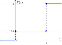
The CDF is a step function when \(X\) can take on only countably many values
Example: \(\mathbb{P}[X=0]=0.25\), \(\mathbb{P}[X=1]=0.75\), and \(\mathbb{P}[X=x]=0\) for \(x\ne 0,1\).

Continuous distributions

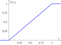
A distribution is continuous if \(F(x)\) is continuous at all \(x\)
In this case, \(\mathbb{P}[X=x] = F(x)- \lim_{u\uparrow x} F(u) = F(x)-F(x)=0\)

Probability Mass and Density Functions (PMF and PDF)

PMF

Discrete random variable \(X\)
Support of the distribution: \(x\in\mathbb R\) such that \(\mathbb{P}[X=x]>0\)
PMF: \(p(x)=\mathbb{P}[X=x]\) for \(x\) in the support
Properties:
- \(p(x)\geq 0\) for all \(x\)
- \(\sum_x p(x)=1\)
- \(F(x)=\sum_{x_i\leq x} p(x_i)\)

Recap: conditioning with a discrete random variable

If \(X\) is discrete with PMF \(p(x_i)=\mathbb{P}[X=x_i]\), the events \(\{X=x_i\}\) partition \(\Omega\)
Total probability and Bayes’ rule then specialize to a discrete \(X\): \[ \mathbb{P}[A]=\sum_i \mathbb{P}[A\mid X=x_i]\,p(x_i),\qquad \mathbb{P}[X=x_i\mid A]=\frac{\mathbb{P}[A\mid X=x_i]\,p(x_i)}{\sum_j \mathbb{P}[A\mid X=x_j]\,p(x_j)} \]

PDF

When a CDF is continuous (and differentiable at \(x\))
Definition of PDF: \(f(x) = \frac{dF(x)}{dx}\)
One can always compute PDF from CDF, and CDF from PDF. They are equivalent descriptions of a continuous distribution
Support of the distribution: \(x\in\mathbb R\) such that \(f(x)>0\)

Properties of PDF

\(f(x)\geq 0\) for all \(x\in\mathbb R\)
\(F(x) =\int_{-\infty}^x f(u)du\)
\(\int_{-\infty}^\infty f(u) du=\lim_{x\to\infty} F(x)=1\)
Note: \(f(x)\) is not a probability and may exceed 1; only areas under the density, \(\int_a^b f(u)\,du=\mathbb{P}[a<X\leq b]\), are probabilities

Recap: conditioning with a density

If \(X\) is continuous with density \(f_X\), the sum over scenarios becomes an integral: \[ \mathbb{P}[A]=\int_{-\infty}^\infty \mathbb{P}[A\mid X=x]\,f_X(x)\,dx \]
Observing an event \(A\) updates the density of \(X\) by Bayes’ rule: \[ f_{X\mid A}(x)=\frac{\mathbb{P}[A\mid X=x]\,f_X(x)}{\int_{-\infty}^\infty \mathbb{P}[A\mid X=t]\,f_X(t)\,dt} \]

Visualizing PMF and PDF

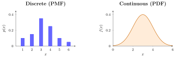
Discrete: probability is concentrated at mass points, \(F(x)=\sum_{x_i\leq x}p(x_i)\)
Continuous: probability is area under the density, \(F(x)=\int_{-\infty}^x f(u)\,du\)

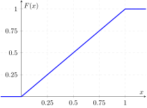
Example: Uniform\((0,1)\) distribution

PDF

\(f(x) =\begin{cases} 0, & x<0\\ 1, & x\in[0,1] \\ 0, & x>1\end{cases}\)

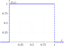
Support: \([0,1]\)

CDF

\(F(x) = \begin{cases} 0, & x < 0 \\ x, & x \in [0,1] \\ 1, & x > 1 \end{cases}\)

Moments

Moments of a distribution

CDF provides a complete description of the behavior of the random variable
May be complicated to work with as it is a function
Moments capture some of the properties and are easier to work with as they are numbers

Expectation operator

The expectation operator is denoted as \({\mathbb{E}}[\cdot]\)
Let \(g:\mathbb R\to\mathbb R\) be a function
- For a discrete \(X\): \({\mathbb{E}}[g(X)] = \sum_i g(x_i) p(x_i)\), where \(p(x_i)=\mathbb{P}[X=x_i]\), and the sum is over all support points \(x_i\)
- For a continuous \(X\): \({\mathbb{E}}[g(X)] = \int g(x) f(x) dx\), where \(f(x)\) is the PDF of \(X\)
Note: The expectation is a property of the distribution (\(p(\cdot)\) or \(f(\cdot)\)), not of the random variable

Discrete random variable \(X\)

Support points: \(x_1,x_2,\ldots\)
PMF: \(p(x_1),p(x_2),\ldots\)
Moment of order \(k=1,2,\ldots\): \({\mathbb{E}}[X^k] = \sum_{i} x_i^k p(x_i)\)

Continuous random variable \(X\)

PDF: \(f(x)\)
Moment of order \(k=1,2,\ldots\): \({\mathbb{E}}[X^k] = \int x^k f(x) dx\)

Existence of moments

We may get \({\mathbb{E}}[X^k]=\infty\) or \({\mathbb{E}}[X^k]=\infty-\infty\), in which case the moment does not exist
Moment of order \(k\) exists if and only if \({\mathbb{E}}[|X|^k]<\infty\)

Interpretation for \(k=1\)

Mean: \({\mathbb{E}}[X]\)
“Center” of the distribution: \({\mathbb{E}}[X] =\arg\min_x {\mathbb{E}}[(X-x)^2]\)

Central moments

Central moment of order \(k\): \({\mathbb{E}}[(X-{\mathbb{E}}[X])^k]\)
For \(k=1\), the central moment is zero
For \(k=2\) the central moment is the variance:
- \(\operatorname{Var}(X)={\mathbb{E}}[(X-{\mathbb{E}}[X])^2]={\mathbb{E}}[X^2]-\big({\mathbb{E}}[X]\big)^2\)
- A measure of dispersion; \(\operatorname{Var}(X)\geq 0\), with equality iff \(X\) is constant (with probability 1)
- Standard deviation: \(\sqrt{\operatorname{Var}(X)}\)

Properties

Linearity: \({\mathbb{E}}[aX+bY]=a\,{\mathbb{E}}[X]+b\,{\mathbb{E}}[Y]\) for constants \(a,b\) (no independence required)
\({\mathbb{E}}[c]=c\) for a constant \(c\)
Monotonicity: if \(X\leq Y\) with probability 1, then \({\mathbb{E}}[X]\leq{\mathbb{E}}[Y]\)
\(\operatorname{Var}(a+bX) = b^2 \operatorname{Var}(X)\)

Common distributions

Mean and variance of some standard distributions:

Distribution	Support	\({\mathbb{E}}[X]\)	\(\operatorname{Var}(X)\)
Bernoulli\((p)\)	\(\{0,1\}\)	\(p\)	\(p(1-p)\)
Binomial\((n,p)\)	\(\{0,1,\ldots,n\}\)	\(np\)	\(np(1-p)\)
Uniform\((a,b)\)	\([a,b]\)	\(\frac{a+b}{2}\)	\(\frac{(b-a)^2}{12}\)
\(\mathcal N(\mu,\sigma^2)\)	\(\mathbb R\)	\(\mu\)	\(\sigma^2\)

Quantiles

Quantile of order \(\tau\in[0,1]\)

Definition: for \(\tau \in [0,1]\), the \(\tau\)-th quantile \(q_\tau\) is the smallest \(x\) such that \(F(x)\geq \tau\)
Interpretation: \(q_\tau\) is the value such that \(\tau\) proportion of the distribution is below it
Example: \(q_{0.5}\) is the median, \(q_{0.25}\) is the first quartile, \(q_{0.75}\) is the third quartile

Quantile as inverse CDF

Suppose CDF \(F(x)\) is strictly increasing: for \(x_1<x_2\), \(F(x_1)<F(x_2)\)
Then \(F\) is invertible: there exists a function \(F^{-1}:(0,1)\to\mathbb R\) such that \(F(F^{-1}(\tau))=\tau\) for all \(\tau\in(0,1)\)
Then \(q_\tau = F^{-1}(\tau)\) is the inverse CDF

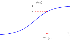
\(\mathbb{P}[X\leq q_\tau] = F(q_\tau) = \tau\)
\(F(q_\tau) = F(F^{-1}(\tau)) = \tau\)

Symmetric distributions

A distribution is symmetric around zero if \(F(x)=1-F(-x)\) for all \(x\in\mathbb R\)
In this case, \(q_\tau = -q_{1-\tau}\) for all \(\tau\in(0,1)\)

Joint/Multivariate distributions

Joint and marginal CDF and PDF

\(X_1,\ldots,X_k\) are random variables on the same probability space
Joint
- CDF: \(F(x_1,\ldots,x_k) = \mathbb{P}[X_1\leq x_1,\ldots,X_k \leq x_k]\)
- PMF (for discrete distribution): \(p(x_1,\ldots,x_k) =\mathbb{P}[X_1= x_1,\ldots,X_k = x_k]\)
- PDF (for continuous distribution): \(f(x_1,\ldots,x_k) =\frac{\partial^k F(x_1,\ldots,x_k)}{\partial x_1\ldots \partial x_k}\)
- Joint behavior of the \(k\) random variables
Marginal
- CDF: \(F_{X_1}(x)=\mathbb{P}[X_1\leq x]\)
- PDF: \(f_{X_1}(x)=\frac{dF_{X_1}(x)}{dx}\)
- Only information about \(X_1\)

From joint to marginal

Let \(F(x_1,x_2)\) be the joint CDF of \(X_1\) and \(X_2\)
- \(F_{X_1}(x)= \mathbb{P}[X_1\leq x,X_2<\infty] = \lim_{u\to\infty} F(x,u)\)
Let \(f(x_1,x_2)\) be the joint PDF of continuous \(X_1\) and \(X_2\)
- \(F_{X_1}({\color{red}x}) =\int_{-\infty}^{\color{red}x} \int_{-\infty}^\infty f(u_1,u_2) d u_2 d u_1\)
- \(f_{X_1}({\color{red}x}) = \frac{d}{d{\color{red}x}}F_{X_1}({\color{red}x}) = \int_{-\infty}^\infty f({\color{red}x},u_2) d u_2\)
For discrete \(X_1,X_2\) with joint PMF \(p(x_1,x_2)\): \(p_{X_1}(x_1)=\sum_{x_2} p(x_1,x_2)\)

Exercise: computing marginal distributions

Joint PMF of discrete \(X_1\in\{1,2\}\) and \(X_2\in\{1,2,3\}\):

\(p(x_1,x_2)\)	\(X_2=1\)	\(X_2=2\)	\(X_2=3\)
\(X_1=1\)	0.10	0.15	0.05
\(X_1=2\)	0.20	0.30	0.20

Compute the marginal PMF \(p_{X_1}(x_1)\) by summing across each row, and \(p_{X_2}(x_2)\) by summing down each column
Check that both marginal PMFs sum to 1

Worked solution

Conditional distributions

Restricting the distribution of one variable to a value of the other:
- Discrete: \(p_{X_2\mid X_1}(x_2\mid x_1)=\dfrac{p(x_1,x_2)}{p_{X_1}(x_1)}\) for \(p_{X_1}(x_1)>0\)
- Continuous: \(f_{X_2\mid X_1}(x_2\mid x_1)=\dfrac{f(x_1,x_2)}{f_{X_1}(x_1)}\) for \(f_{X_1}(x_1)>0\)
This is the random-variable analogue of \(\mathbb{P}[A\mid B]=\mathbb{P}[A\cap B]/\mathbb{P}[B]\)

Independence

\(X_1\) and \(X_2\) are independent iff the joint CDF is the product of the marginal CDFs: \(F(x_1,x_2)=F_{X_1}(x_1)F_{X_2}(x_2)\) for all \(x_1,x_2\)
Equivalently for continuous random variables iff the joint PDF is the product of the marginal PDFs: \(f(x_1,x_2)=f_{X_1}(x_1)f_{X_2}(x_2)\) for all \(x_1,x_2\)
Equivalently for discrete random variables iff the joint PMF factors: \(p(x_1,x_2)=p_{X_1}(x_1)p_{X_2}(x_2)\) for all \(x_1,x_2\)

Joint moments

Let \(X_1,X_2\) be continuously distributed with a pdf \(f(x_1,x_2)\)
\({\mathbb{E}}[g(X_1,X_2)] = \int_{-\infty}^\infty \int_{-\infty}^\infty g(x_1,x_2) f(x_1,x_2) dx_2 dx_1\)

Covariance

\[ \begin{aligned} \operatorname{Cov}(X_1,X_2) &= {\mathbb{E}}[(X_1-{\mathbb{E}}[X_1])(X_2-{\mathbb{E}}[X_2])] \\ &= \int_{-\infty}^\infty \int_{-\infty}^\infty (x_1-{\mathbb{E}}[X_1])(x_2-{\mathbb{E}}[X_2])f(x_1,x_2) dx_2 dx_1 \end{aligned} \]

Computational formula: \(\operatorname{Cov}(X_1,X_2)={\mathbb{E}}[X_1 X_2]-{\mathbb{E}}[X_1]\,{\mathbb{E}}[X_2]\)
Sign: \(\operatorname{Cov}(X_1,X_2)>0\) means \(X_1,X_2\) tend to move together; \(<0\) opposite directions; \(=0\) uncorrelated
\(\operatorname{Cov}(X,X)={\mathbb{E}}[X^2]-\big({\mathbb{E}}[X]\big)^2=\operatorname{Var}(X)\)

Properties

\(\operatorname{Cov}(c,X) =0\)
\(\operatorname{Cov}(bX_1,cX_2)=bc\operatorname{Cov}(X_1,X_2)\)
\(\operatorname{Var}(a+bX_1+cX_2)=b^2 \operatorname{Var}(X_1)+c^2\operatorname{Var}(X_2)+2bc\operatorname{Cov}(X_1,X_2)\)
If \(X_1,X_2\) are independent, then \({\mathbb{E}}[X_1X_2]={\mathbb{E}}[X_1]{\mathbb{E}}[X_2]\), \(\operatorname{Cov}(X_1,X_2)=0\), and \(\operatorname{Var}(X_1+X_2)=\operatorname{Var}(X_1)+\operatorname{Var}(X_2)\)
The converse is false: \(\operatorname{Cov}(X_1,X_2)=0\) does not imply independence

Correlation

Definition: \[ \operatorname{Corr}(X_1,X_2)=\frac{\operatorname{Cov}(X_1,X_2)}{\sqrt{\operatorname{Var}(X_1)\,\operatorname{Var}(X_2)}} \]
A unitless (scale-free) measure of linear association
\(-1\leq\operatorname{Corr}(X_1,X_2)\leq 1\) (a consequence of the Cauchy–Schwarz inequality, shown later)
\(|\operatorname{Corr}(X_1,X_2)|=1\) iff \(X_2=a+bX_1\) for some constants \(a,b\)

Conditional expectation

Let \(X\) and \(Y\) be two random variables. The conditional expectation of \(Y\) given \(X=x\) uses the conditional distribution of \(Y\) given \(X=x\):
- Discrete: \({\mathbb{E}}[Y\mid X=x]=\sum_y y\,p_{Y\mid X}(y\mid x)\)
- Continuous: \({\mathbb{E}}[Y\mid X=x]=\int_{-\infty}^\infty y\,f_{Y\mid X}(y\mid x)\,dy\)
It produces a number for each value \(x\)

Conditional expectation as a random variable

\({\mathbb{E}}[Y\mid X=x]\) is a function of \(x\); write \(g(x)={\mathbb{E}}[Y\mid X=x]\)
Then \({\mathbb{E}}[Y\mid X]=g(X)\) is itself a random variable, inheriting its randomness from \(X\)
Two distinct objects:
- \({\mathbb{E}}[Y\mid X=x]\): a number, for a specific value \(x\)
- \({\mathbb{E}}[Y\mid X]\): a random variable, a function of \(X\)

Exercise: computing \({\mathbb{E}}[Y\mid X]\)

\(X\in\{0,1\}\) and \(Y\in\{0,1,2\}\) with joint PMF:

\(p(x,y)\)	\(Y=0\)	\(Y=1\)	\(Y=2\)
\(X=0\)	0.10	0.20	0.10
\(X=1\)	0.05	0.25	0.30

Compute \({\mathbb{E}}[Y\mid X=0]\) and \({\mathbb{E}}[Y\mid X=1]\), and express \({\mathbb{E}}[Y\mid X]\) as a function of \(X\)

Worked solution

Unifying two notations

Two conditional expectations that look different:
- \({\mathbb{E}}[X\mid Y]\): given \(Y\) takes some value
- \({\mathbb{E}}[X\mid X<y]\): given \(X\) is below a threshold \(y\)
The second is a special case of the first. Define the indicator \(D=\mathbb{1}\{X<y\}\); then \[ {\mathbb{E}}[X\mid X<y]={\mathbb{E}}[X\mid D=1] \]
In both cases, conditioning restricts the distribution to a subset, and the expectation is taken over the restricted distribution

\({\mathbb{E}}[X\mid X<y]\) in integral form

For continuous \(X\) with density \(f_X\), \[ {\mathbb{E}}[X\mid X<y]=\frac{\int_{-\infty}^y x\,f_X(x)\,dx}{\int_{-\infty}^y f_X(x)\,dx}=\frac{\int_{-\infty}^y x\,f_X(x)\,dx}{F_X(y)} \]
The numerator integrates \(x\,f_X(x)\) only over \(\{X<y\}\); the denominator \(F_X(y)=\mathbb{P}[X<y]\) renormalizes so the conditional density integrates to 1
Conditional density: \(f_{X\mid X<y}(x)=f_X(x)/F_X(y)\) for \(x<y\), and \(0\) otherwise

Why conditional expectation matters

In econometrics, objects like \({\mathbb{E}}[\text{Wage}\mid \text{Employed}=1]={\mathbb{E}}[\text{Wage}\mid D=1]\) with \(D=\mathbb{1}\{\text{Employed}\}\) are everywhere
The selection problem: \({\mathbb{E}}[\text{Wage}\mid D=1]\neq{\mathbb{E}}[\text{Wage}]\) whenever employment status is correlated with potential wages
Viewing every conditional expectation as \({\mathbb{E}}[\,\cdot\mid \text{some RV}=\text{some value}]\) gives a unified framework

Properties of conditional expectation

Linearity: \({\mathbb{E}}[aY+bZ\mid X]=a\,{\mathbb{E}}[Y\mid X]+b\,{\mathbb{E}}[Z\mid X]\)
Taking out what is known: \({\mathbb{E}}[g(X)\,Y\mid X]=g(X)\,{\mathbb{E}}[Y\mid X]\)
Independence: if \(Y\) and \(X\) are independent, \({\mathbb{E}}[Y\mid X]={\mathbb{E}}[Y]\)
Tower property: \({\mathbb{E}}\big[{\mathbb{E}}[Y\mid X]\big]={\mathbb{E}}[Y]\) (next section)

Practice: Taking Out What Is Known

Practice: Taking out what is known

Prove the “taking out what is known” property for discrete random variables: for any function \(g\), \[ {\mathbb{E}}[g(X)\,Y \mid X] = g(X)\,{\mathbb{E}}[Y \mid X]. \]

Worked solution

Law of iterated expectations

For any random variables \(X\) and \(Y\), \[ {\mathbb{E}}[Y]={\mathbb{E}}\big[{\mathbb{E}}[Y\mid X]\big] \]
Intuition: \({\mathbb{E}}[Y\mid X]\) is the local average of \(Y\) for each value of \(X\); averaging these local averages over the distribution of \(X\) recovers the overall average
Discrete form: \({\mathbb{E}}[Y]=\sum_x {\mathbb{E}}[Y\mid X=x]\,p_X(x)\)

Exercise: LIE in action

A course has two sections: A has 30 students averaging 72; B has 20 students averaging 80
Let \(S\) be the section and \(G\) the grade, so \({\mathbb{E}}[G\mid S=A]=72\) and \({\mathbb{E}}[G\mid S=B]=80\)
Use the law of iterated expectations to find \({\mathbb{E}}[G]\)

Worked solution

Exercise: verifying the LIE by direct computation

Return to the joint PMF from the earlier exercise (\(X\in\{0,1\}\), \(Y\in\{0,1,2\}\)):

\(p(x,y)\)	\(Y=0\)	\(Y=1\)	\(Y=2\)
\(X=0\)	0.10	0.20	0.10
\(X=1\)	0.05	0.25	0.30

Compute \({\mathbb{E}}[Y]\) two ways and check that they agree:
1. Directly: sum the joint table over \(x\) to get the marginal PMF \(p_Y(y)\), then compute \({\mathbb{E}}[Y]=\sum_y y\,p_Y(y)\)
2. Via the LIE: using \({\mathbb{E}}[Y\mid X=0]\) and \({\mathbb{E}}[Y\mid X=1]\) from the earlier exercise, and the marginal \(p_X(x)\), compute \({\mathbb{E}}[Y]={\mathbb{E}}[Y\mid X=0]\,p_X(0)+{\mathbb{E}}[Y\mid X=1]\,p_X(1)\)

Worked solution

LIE with multiple conditioning variables

Conditioning on two variables \(X\) and \(Z\): \[ {\mathbb{E}}\big[{\mathbb{E}}[Y\mid X,Z]\,\big|\,X\big]={\mathbb{E}}[Y\mid X] \]
The inner expectation conditions on both \(X\) and \(Z\); the outer averages out \(Z\) while holding \(X\) fixed
The “most information” is on the inside; the outer expectation peels off one layer

Where the LIE appears

Econometrics: the engine behind “controlling for” covariates. If you want \({\mathbb{E}}[Y\mid X]\) but also observe \(Z\), \[ {\mathbb{E}}[Y\mid X]={\mathbb{E}}\big[{\mathbb{E}}[Y\mid X,Z]\,\big|\,X\big] \] condition on everything, then average out what is not needed
Dynamic programming: with \({\mathbb{E}}_t[\cdot]={\mathbb{E}}[\cdot\mid \mathcal I_t]\) the information at time \(t\), the tower property gives \({\mathbb{E}}_t\big[{\mathbb{E}}_{t+1}[Y]\big]={\mathbb{E}}_t[Y]\)

Useful inequalities

Markov’s Inequality

Let \(X\) be a non-negative random variable (\(X \geq 0\)) and \(a > 0\)

\[ \mathbb{P}[X \geq a] \leq \frac{{\mathbb{E}}[X]}{a} \]

Interpretation: Bounds the tail probability using the moment
Proof Sketch: Let \(\mathbb{1}(\cdot)\) be the indicator function that takes the value 1 if the condition is true and 0 otherwise. Then, \({\mathbb{E}}[X] = {\mathbb{E}}[X \cdot \mathbb{1}(X \geq a)] + {\mathbb{E}}[X \cdot \mathbb{1}(X < a)] \geq a \mathbb{P}[X \geq a]\)

Cauchy-Schwarz Inequality

For random variables \(X\) and \(Y\) with finite second moments:

\[ |{\mathbb{E}}[XY]| \leq \sqrt{{\mathbb{E}}[X^2] {\mathbb{E}}[Y^2]} \]

Equality: Holds if \(X\) and \(Y\) are linearly dependent (i.e., \(Y = cX\) for some constant \(c\))
Covariance form: \(|\operatorname{Cov}(X,Y)|\leq\sqrt{\operatorname{Var}(X)\,\operatorname{Var}(Y)}\), which gives the correlation bound \(|\operatorname{Corr}(X,Y)|\leq 1\)
Proof Follows from the fact that \({\mathbb{E}}[(X + \lambda Y)^2] \geq 0\) for all \(\lambda\).

Practice: Proving Cauchy–Schwarz

Practice: Prove the Cauchy–Schwarz inequality

Show that \(\big({\mathbb{E}}[XY]\big)^2 \leq {\mathbb{E}}[X^2]\,{\mathbb{E}}[Y^2]\) for random variables with finite second moments.

Hint: expand \({\mathbb{E}}[(X - tY)^2] \geq 0\) as a quadratic in \(t\) and use its discriminant.

Worked solution

Proof of Cauchy-Schwarz Inequality

Let \(X\) and \(Y\) be random variables with finite second moments. For any real number \(\lambda\), consider the non-negative expectation: \({\mathbb{E}}[(X + \lambda Y)^2] \geq 0\). Expanding, \({\mathbb{E}}[(X + \lambda Y)^2] = {\mathbb{E}}[X^2] + 2\lambda {\mathbb{E}}[XY] + \lambda^2 {\mathbb{E}}[Y^2]\). This quadratic in \(\lambda\) must be non-negative for all \(\lambda\), so its discriminant is non-positive: \((2{\mathbb{E}}[XY])^2 - 4{\mathbb{E}}[X^2]{\mathbb{E}}[Y^2] \leq 0\), so \(4({\mathbb{E}}[XY])^2 \leq 4{\mathbb{E}}[X^2]{\mathbb{E}}[Y^2]\), and thus \(|{\mathbb{E}}[XY]| \leq \sqrt{{\mathbb{E}}[X^2]{\mathbb{E}}[Y^2]}\).

Jensen’s Inequality

Let \(X\) be a random variable and \(\phi(\cdot)\) a convex function

\[ {\mathbb{E}}[\phi(X)] \geq \phi({\mathbb{E}}[X]) \]

Equality: Holds if \(X\) is constant or \(\phi\) is linear
Example: For \(\phi(x) = x^2\), \({\mathbb{E}}[X^2] \geq ({\mathbb{E}}[X])^2\)
If \(\phi\) is concave, the inequality is reversed: \({\mathbb{E}}[\phi(X)] \leq \phi({\mathbb{E}}[X])\)

Where these inequalities appear

Jensen: risk aversion in micro/macro (concave utility): \({\mathbb{E}}[\phi(W)]\leq \phi({\mathbb{E}}[W])\) for a risk-averse agent
Markov: building block for Chebyshev’s inequality and convergence results
Cauchy–Schwarz: bounding correlations; efficiency bounds for estimators (Cramér–Rao)