Show the code
# !pip install matplotlib numpy pandas opencv-python scikit-learn torch torchvision transformers datasets grad-cam tensorflow kerasIn this notebook you will
Before you start, make sure you
.zip files.# !pip install matplotlib numpy pandas opencv-python scikit-learn torch torchvision transformers datasets grad-cam tensorflow kerasImportant: Please run the following cells before continuing, as it sets up the libraries and image folders required for this notebook.
# Library loading

# Standard library
import os
from collections import defaultdict
from pathlib import Path

# Imaging / computer vision
from PIL import Image
import cv2
import numpy as np
from torchvision import transforms

# Visualization
import matplotlib.pyplot as plt
from mpl_toolkits.mplot3d import Axes3D
from matplotlib.colors import ListedColormap
import plotly.express as px
import plotly.io as pio

# Data handling
import pandas as pd

# SciPy / numerical utilities
from scipy.ndimage import convolve

# scikit-learn
from sklearn.cluster import KMeans
from sklearn.decomposition import PCA
from sklearn.metrics.pairwise import cosine_similarity
from sklearn.preprocessing import LabelEncoder
from sklearn.datasets import make_moons
from sklearn.model_selection import train_test_split
from sklearn.linear_model import LogisticRegression
from sklearn.neural_network import MLPClassifier
from sklearn import metrics
from sklearn.metrics import classification_report

# TensorFlow / Keras (VGG16)
from tensorflow.keras.applications import VGG16
from tensorflow.keras.preprocessing import image as keras_image
from tensorflow.keras.applications.vgg16 import preprocess_input

# PyTorch / torchvision / transformers
import torch
import torch.nn as nn
import torch.optim as optim
from torch.utils.data import Dataset, DataLoader
from torch.utils.data import random_split
from torchvision.models import convnext_base, ConvNeXt_Base_Weights
from transformers import AutoImageProcessor, ConvNextV2Model

# Misc
from tqdm.notebook import tqdm

# Local helpers
from data.zip_extractor import ZipExtractor# Don't change this cell
# Define the source path and the destination
sources = ["example_images.zip", "richter_kouroi_complete_front_only.zip"]
dest = "data/"
for src in sources:
extractor = ZipExtractor(src, dest)
extractor.extract_all()Extracted 'example_images.zip' to 'data\example_images'
Extracted 'richter_kouroi_complete_front_only.zip' to 'data\richter_kouroi_complete_front_only'In this notebook, we explore a dataset of photographs collected from Gisela Richter’s Kouroi: Archaic Greek Youths: a Study of the Development of the Kouros Type in Greek Sculpture (1942).
Gisela Richter’s 1942 book was one of the first systematic efforts to catalog and classify kouroi based on their stylistic evolution. Her work combined archaeological evidence with visual comparison, laying the foundation for how we study ancient sculpture today.
In this project, we aim to apply computer vision techniques to digitally analyze and group images from this dataset. Just as Richter used her trained eye to identify patterns and typologies, we’ll explore how machines can “see” these sculptures through their eyes (image embeddings, clustering, and convolutional neural networks).
Have you ever wondered how images are stored in computers, how computers see them and distinguish the difference between them?
Many of you probably know that digital images are stored based on pixels as a grid of figures, but when we are doing image searches using a search engine or uploading them to a Generative AI model, how exactly do computers interpret, distinguish, and process them? Here is a brief introduction to some of the basic forms and methods.
Have you ever heard of the RGB primary colour model? For those who are unfamiliar with the concept, the model uses numbers in a range 0 ~ 255 to represent the colour intensity of red, green and blue and add up the three colour channels to generate any colour that’s visible to humans. In a colorful digital image, each pixel is characterized by its colour stored in the form (R, G, B), so knowing the distribution of colour intensity gives you a lot of information about the image.
However, for monochrome images, there is only one colour channel, the grayscale. We can still use the distribution of grayscale intensities to represent the image. Since all of our images (cropped from scanned pdf books) are printed in monochrome, we can represent them using a grayscale colour histogram.
Let’s start with a three-view of the New York Kouros, here we read in the images and present them together.
# Define the folder path where the images are stored
image_path = 'data/example_images'

fig, axes = plt.subplots(1, 3, figsize=(8, 5))

# List of specific image filenames
image_names = {'page188_img01_photo12.jpg': "Left", 'page188_img01_photo13.jpg': "Front", 'page189_img01_photo3.jpg': "Back"}

# Display the images side by side
axes = axes.flatten()
for i, img_name in enumerate(image_names):
    img_path = f"{image_path}/{img_name}"
    image = Image.open(img_path)
    axes[i].imshow(image)
    axes[i].set_title(image_names[img_name])
    axes[i].axis('off')

plt.suptitle("Selected Images from Richter's Kouroi Dataset")
plt.tight_layout()
plt.show()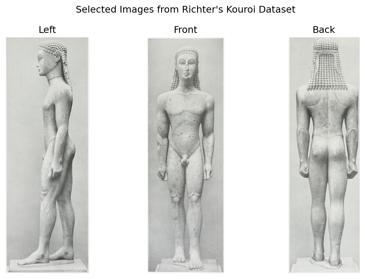
Each of these images, when loaded into the computer, becomes a 2D array of numbers representing intensity values. We then plot the colour histogram for each image representing the distribution of grayscale intensity.
Discussion: What do you notice by looking at the three histograms?
# Generate and plot greyscale histograms for the selected images
fig, axes = plt.subplots(1, 3, figsize=(7, 4))

for i, img_name in enumerate(image_names):
    img_path = f"{image_path}/{img_name}"
    image = Image.open(img_path)
    histogram = image.histogram()

    axes[i].plot(histogram, color='black')
    axes[i].set_title(f'{image_names[img_name]}')
    axes[i].set_xlim([0, 255])
    axes[i].set_xlabel("Intensity")
    if i == 0:
        axes[i].set_ylabel("Frequency")

plt.tight_layout()
plt.show()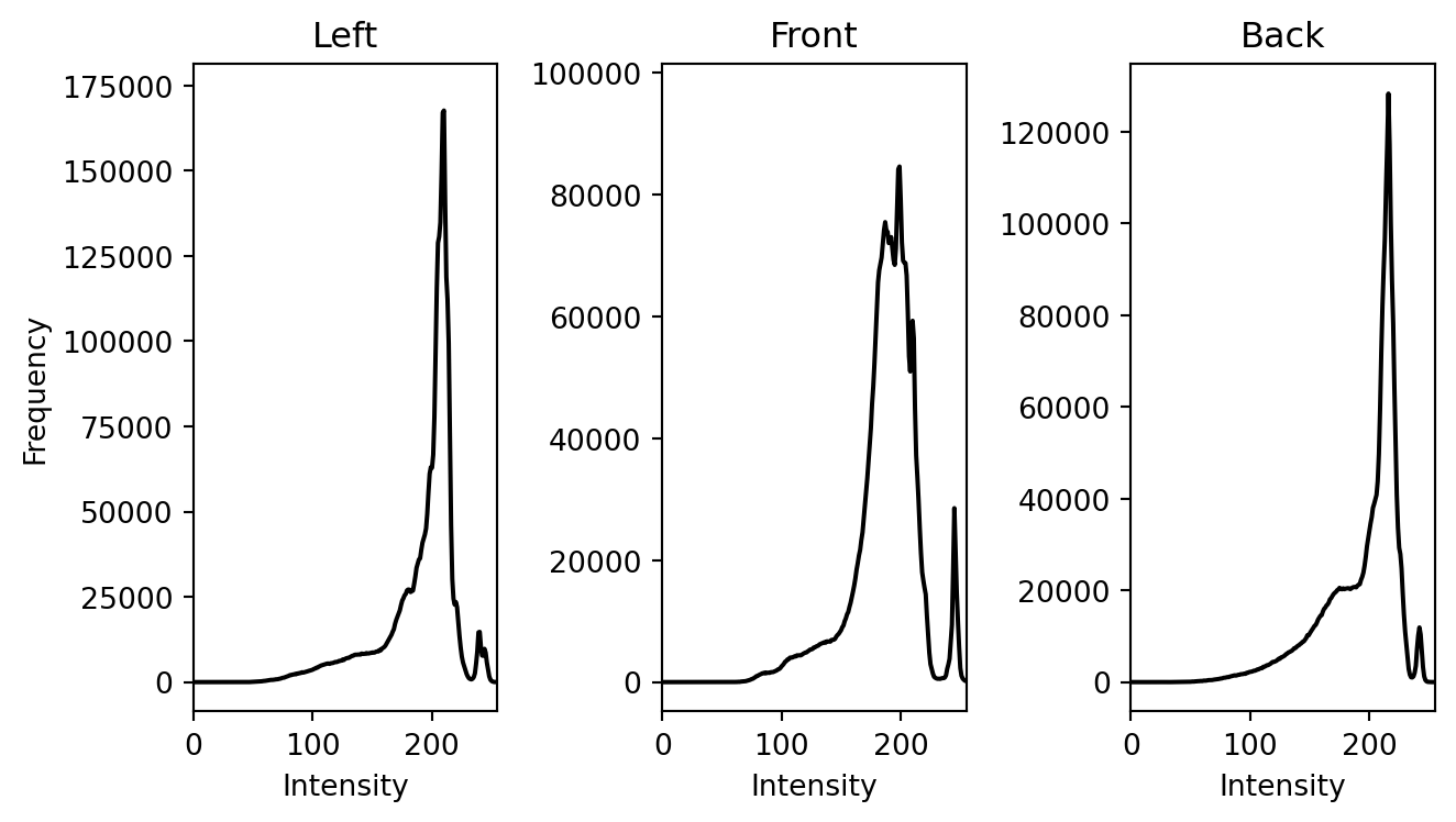
They look very similar! This result is not surprising given that the three images were taken at the same time with the same equipment of the same Kouros. The above example shows us that comparing the similarity of colour distributions is one way that computers understand the similarity of images.
However, one can quickly realize the drawbacks of this approach. First, it relies on the correct representation of colour, so two identical images with colour differences may not be recognized as similar. Second, since it focuses only on colour, it ignores the fundamental information for object recognition such as spatial, shape and texture in the image. Last but not least, there may exist two completely different images with exactly the same color distribution. Therefore, we need better methods to consider the similarity between images.
Bag of Visual Words (BoVW) is a more practical method for recognizing similarity. The rationale behind this is very complicated, but to put it simply, it treats a “feature” in an image as a “word” (a set of numbers containing information about the feature) and calculates how often each word appears in the image. Here, we created a visual vocabulary containing 20 “words” using three-view photos of the New York Kouros, and visualized what a visual word represents on the left-view image. Here, we pick the visual word with ID 6:
# Define the number of clusters for KMeans
n_clusters   = 20
word_to_show = 6
max_patches  = 30

# Initialize ORB detector
orb = cv2.ORB_create(nfeatures=500)
all_descriptors = []      # for stacking
image_data      = []      # (img_name, kps, descs)

# Detect and describe all images
for img_name in image_names:
    img_path = os.path.join(image_path, img_name)
    img      = cv2.imread(img_path, cv2.IMREAD_GRAYSCALE)
    keypoints, descriptors = orb.detectAndCompute(img, None)

    if descriptors is None:
        descriptors = np.zeros((0, orb.descriptorSize()), dtype=np.uint8)

    all_descriptors.append(descriptors)
    image_data.append((img_name, keypoints, descriptors))

# Build the visual vocabulary
all_descriptors_stacked = np.vstack(all_descriptors)
kmeans = KMeans(n_clusters=n_clusters, random_state=42)
kmeans.fit(all_descriptors_stacked)

# Compute BoVW histograms
histograms = []
for img_name, _, descriptors in image_data:
    if descriptors.shape[0] > 0:
        words = kmeans.predict(descriptors)
        hist, _ = np.histogram(words, bins=np.arange(n_clusters + 1))
    else:
        hist = np.zeros(n_clusters, dtype=int)
    histograms.append((img_name, hist))

# Find the locations matching visual word ID = 6
locations = []
for img_idx, (_, keypoints, descriptors) in enumerate(image_data):
    if descriptors.shape[0] == 0:
        continue
    assignments = kmeans.predict(descriptors)
    for kp, w in zip(keypoints, assignments):
        if w == word_to_show:
            x, y = map(int, kp.pt)
            locations.append((img_idx, x, y))
            if len(locations) >= max_patches:
                break
    if len(locations) >= max_patches:
        break

# Group by image and visualize
imgs = defaultdict(list)
for idx, x, y in locations:
    imgs[idx].append((x, y))

if imgs:
    img_idx, pts = next(iter(imgs.items()))
    fname = image_data[img_idx][0]
    img   = cv2.imread(os.path.join(image_path, fname), cv2.IMREAD_GRAYSCALE)
    img_rgb = cv2.cvtColor(img, cv2.COLOR_GRAY2RGB)
    for x, y in pts:
        cv2.circle(img_rgb, (x, y), radius=25, color=(0,255,0), thickness=2)

    plt.figure(figsize=(6,6))
    plt.imshow(img_rgb)
    plt.title(f"Word {word_to_show} Keypoints on the Left-View Photo")
    plt.axis('off')
    plt.tight_layout()
    plt.show()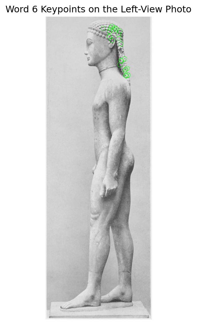
We note that the word “6” could represent the beads in the beadwork worn by the Kouros.
Discussion: Based on your knowledge of the various Kouros, do you think this visual word can be the key to differentiating between different Kouros, or even different sculptural subjects?
As you may have realized, the visual word frequency distributions of different images are not exactly the same, so how can we determine if these images are similar? More importantly, what can we use as a criterion to categorize different images based on visual words? Here, we will use something called cosine similarity to make a measurement.
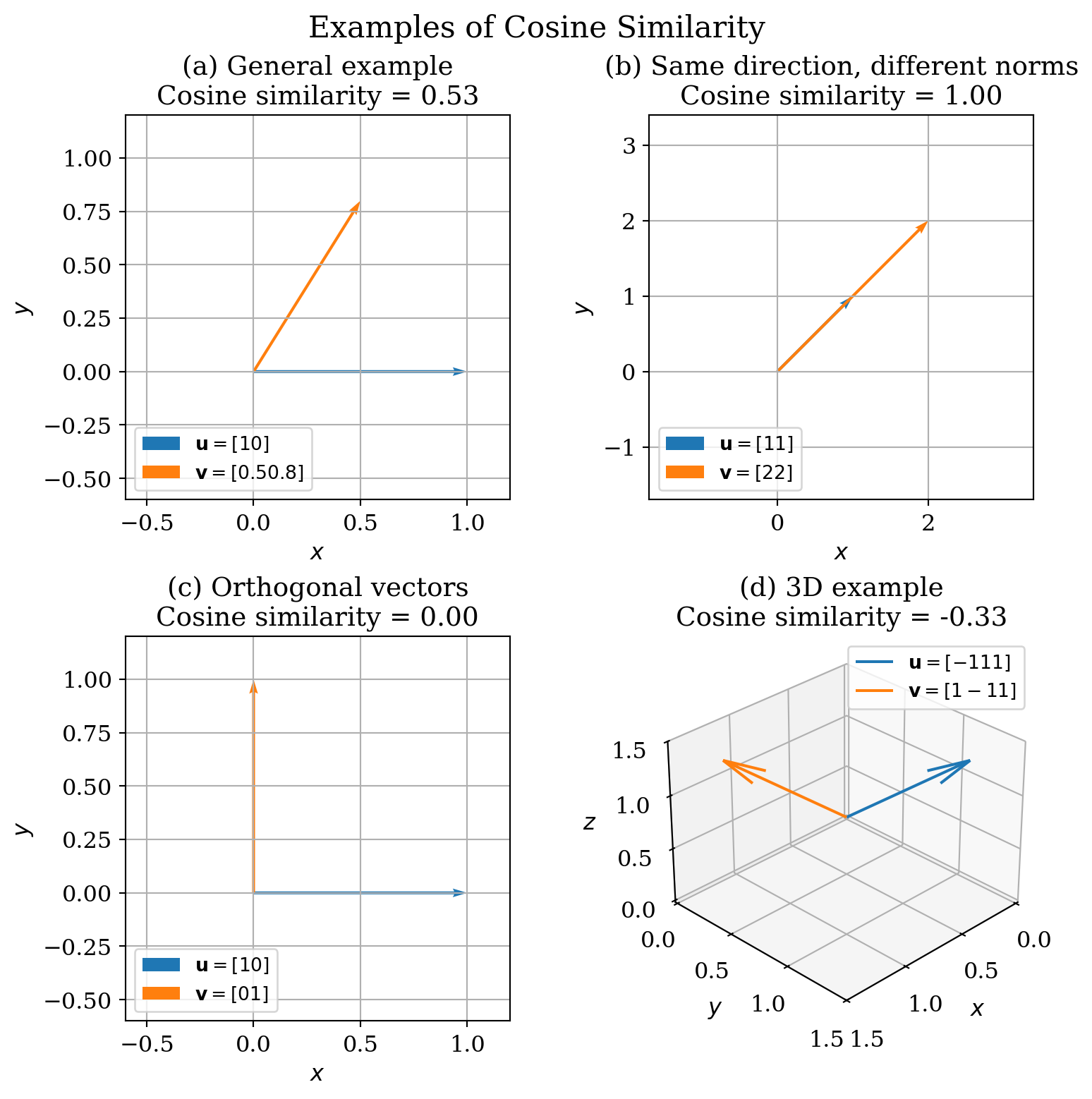
You can think of the visual word frequency histogram for each image as an arrow in space, and cosine similarity is a measure of how much those arrows are pointing in the same direction. The criterion is very intuitive: the closer the cosine similarity of two images is to 1, the more similar the two images are; the closer the cosine similarity is to 0, the less similar the two images are.
Here, we perform pairwise cosine similarity measurements on left-view, front-view, and back-view photographs of New York Kouros, and show the results.
hist_list = []
for img_name, _, descriptors in image_data:
    if descriptors.shape[0] > 0:
        words = kmeans.predict(descriptors)
        hist, _ = np.histogram(words, bins=np.arange(n_clusters + 1))
    else:
        hist = np.zeros(n_clusters, dtype=int)
    hist = hist.astype(float)
    if hist.sum() > 0:
        hist /= hist.sum()
    hist_list.append(hist)

histograms = np.array(hist_list)

sim_matrix = cosine_similarity(histograms)

image_keys = list(image_names.keys())
image_labels = list(image_names.values())

# Display the similarity matrix
fig, ax = plt.subplots(figsize=(8, 5))
cax = ax.imshow(sim_matrix, interpolation='nearest', cmap='viridis')
ax.set_title('BoVW Cosine Similarity between Images')
ax.set_xticks(np.arange(len(image_labels)))
ax.set_yticks(np.arange(len(image_labels)))
ax.set_xticklabels(image_labels, rotation=45, ha='right')
ax.set_yticklabels(image_labels)
fig.colorbar(cax, ax=ax, label='Cosine Similarity')
plt.tight_layout()
plt.show()

print("Pairwise Cosine Similarity Matrix:")
for i in range(len(image_labels)):
    for j in range(i + 1, len(image_labels)):
        print(f"{image_labels[i]} vs {image_labels[j]}: {sim_matrix[i, j]:.3f}")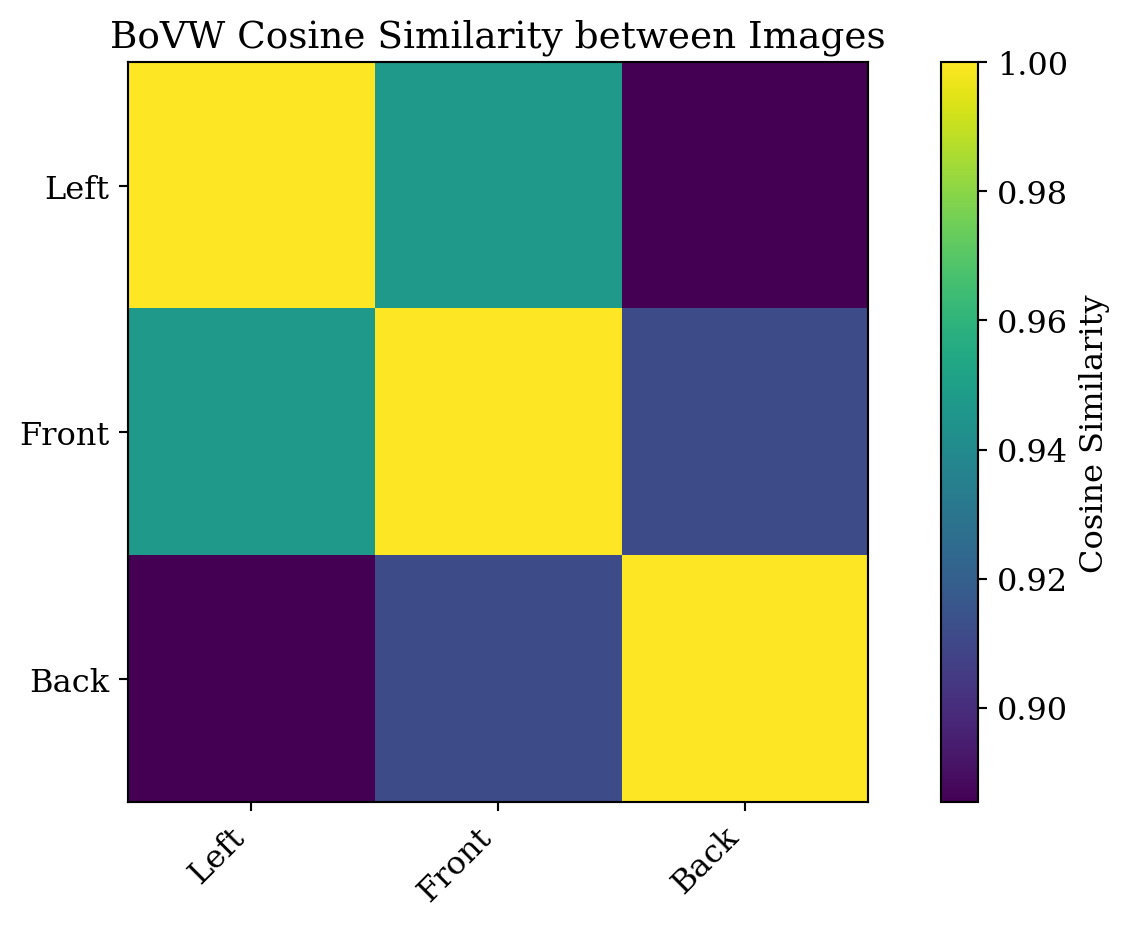
Pairwise Cosine Similarity Matrix:
Left vs Front: 0.947
Left vs Back: 0.885
Front vs Back: 0.912
As you can see, the pairwise cosine similarities are all very high, even though the BoVW histograms look very different! This is good evidence that they are photographs of the same object, and computers can understand this by setting the appropriate threshold.
However, would this also work for photos of different objects? Let’s find out by calculating the cosine similarity between existing images and another Kouros currently exhibited in the Piraeus Archaeological Museum.
# Define a new image to compare with the existing ones
new_image_path = 'data/richter_kouroi_complete_front_only/page312_img01_photo4.jpg'
new_image_label = 'A Kouros from Athens' # Suppose this is a new artifact we just discovered

img_new = cv2.imread(new_image_path, cv2.IMREAD_GRAYSCALE)
orb = cv2.ORB_create(nfeatures=500)
kp_new, desc_new = orb.detectAndCompute(img_new, None)

if desc_new is not None and len(desc_new) > 0:
    words_new = kmeans.predict(desc_new)
    hist_new, _ = np.histogram(words_new, bins=np.arange(kmeans.n_clusters + 1))
else:
    hist_new = np.zeros(kmeans.n_clusters, dtype=int)

hist_new = hist_new.astype(float)
if hist_new.sum() > 0:
    hist_new /= hist_new.sum()

sims = cosine_similarity(histograms, hist_new.reshape(1, -1)).flatten()

# Print the cosine similarity of the new image with existing images
print(f"\nCosine Similarity of '{new_image_label}' with existing images:")
for i, label in enumerate(image_labels):
    print(f"{label} vs {new_image_label}: {sims[i]:.3f}")

# Show the new image
plt.figure(figsize=(5, 5))
plt.imshow(img_new, cmap='gray')
plt.title(f"{new_image_label}")
plt.axis('off')
plt.show()
Cosine Similarity of 'A Kouros from Athens' with existing images:
Left vs A Kouros from Athens: 0.816
Front vs A Kouros from Athens: 0.892
Back vs A Kouros from Athens: 0.839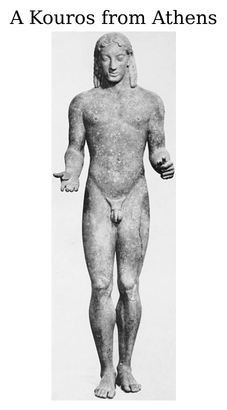
By looking at the results, we see that it has a lower but still relatively high cosine similarity to the previous images, albeit with different textures and poses. Although computers do not understand what “Kouroi” are simply by collecting visual words, they can still see the similarity! To support this view, let’s look at an example that is also a standing figure, but from a different culture (China, Sanxingdui). If our conjecture is correct, its cosine similarity to the previous images will decrease significantly.
# Define a new image to compare with the existing ones
new_image_path2 = 'data/example_images/sanxingdui.jpeg'
new_image_label2 = 'A Bronze Figure from Sanxingdui' # Suppose this is a new artifact we just discovered

img_new2 = cv2.imread(new_image_path2, cv2.IMREAD_GRAYSCALE)
orb = cv2.ORB_create(nfeatures=500)
kp_new, desc_new = orb.detectAndCompute(img_new2, None)

if desc_new is not None and len(desc_new) > 0:
    words_new = kmeans.predict(desc_new)
    hist_new, _ = np.histogram(words_new, bins=np.arange(kmeans.n_clusters + 1))
else:
    hist_new = np.zeros(kmeans.n_clusters, dtype=int)

hist_new = hist_new.astype(float)
if hist_new.sum() > 0:
    hist_new /= hist_new.sum()

sims = cosine_similarity(histograms, hist_new.reshape(1, -1)).flatten()

# Print the cosine similarity of the new image with existing images
print(f"\nCosine Similarity of '{new_image_label2}' with existing images:")
for i, label in enumerate(image_labels):
    print(f"{label} vs {new_image_label2}: {sims[i]:.3f}")

# Show the new image
plt.figure(figsize=(5, 5))
plt.imshow(img_new2, cmap='gray')
plt.title(f"{new_image_label2}")
plt.axis('off')
plt.show()
Cosine Similarity of 'A Bronze Figure from Sanxingdui' with existing images:
Left vs A Bronze Figure from Sanxingdui: 0.586
Front vs A Bronze Figure from Sanxingdui: 0.640
Back vs A Bronze Figure from Sanxingdui: 0.638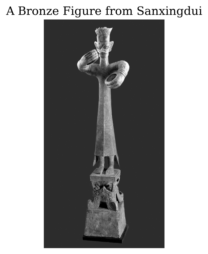
The results were exactly as we expected. The cosine similarity measured for different artistic styles, different poses and different angles of the Sanxingdui sculpture is significantly lower.
This provides us with a hint on how to build an automatic image-based classifier for art and artifacts of different genres, cultures, and textures. Although BoVW also has some obvious limitations (lack of spatial relationships, lack of ability to detect specific objects in complex images), the examples above demonstrate the fundamentals of computer vision, and with the help of more advanced techniques we can do much more in analyzing artwork based on digitized images.
Before diving into applying a convolutional neural network, let’s first make an intuitive introduction to the concept convolution.
Imagine sliding a tiny image over an image as a filter to make the actual image appear the same as the filter. Convolution is the mathematical operation to achieve such an effect.
Below is one of such filters, or its professional term, a kernel, how do you think it will filter an image to make the image look like it?
# Kernel
kernel = np.array([
    [-1, -1, -1],
    [ 0,  0,  0],
    [ 1,  1,  1]
])

# Map: 1 -> 1.0 (white), 0 -> 0.0 (black), -1 -> 1.0 (white)
display_kernel = np.where(kernel == 0, 0, 1)

fig, ax = plt.subplots()
cax = ax.matshow(display_kernel, cmap='gray', vmin=0, vmax=1)
plt.colorbar(cax)

# Annotate the kernel values

ax.set_title('Example of a Kernel')
plt.show()
This is how an actual image convolved with the filter:
# Load the image as grayscale
img_path = "data/example_images/page300_img01_photo8.jpg"
image = Image.open(img_path).convert('L')
img_array = np.array(image)

# Define the horizontal edge detection kernel
kernel = np.array([
    [-1, -1, -1],
    [ 0,  0,  0],
    [ 1,  1,  1]
])

# Convolve the image with the kernel
convolved = convolve(img_array, kernel, mode='reflect')

# Display the original and convolved images
fig, ax = plt.subplots(1, 2, figsize=(8, 4))
ax[0].imshow(img_array, cmap='gray')
ax[0].set_title("Original Image")
ax[0].axis('off')
ax[1].imshow(convolved, cmap='gray')
ax[1].set_title("Convolved with Kernel")
ax[1].axis('off')
plt.show()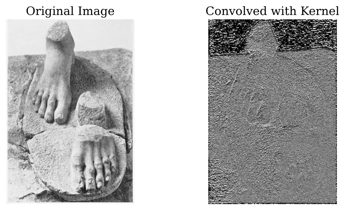
The above is just one example of a convolutional kernel that extracts horizontal edges in an image. In fact, there are many different kernels with different effects. For example, here is a filter that blurs all images:
img = np.array(Image.open(img_path).convert('L'))

def gaussian_kernel(size=21, sigma=5):
    ax = np.linspace(-(size-1)//2, (size-1)//2, size)
    xx, yy = np.meshgrid(ax, ax)
    kernel = np.exp(-(xx**2 + yy**2) / (2. * sigma**2))
    return kernel / np.sum(kernel)

kernel = gaussian_kernel(21, 5)
conv = convolve(img, kernel)
fig, ax = plt.subplots(1, 3, figsize=(8, 3))
ax[0].imshow(img, cmap='gray'); ax[0].set_title("Original"); ax[0].axis('off')
ax[1].imshow(kernel, cmap='gray'); ax[1].set_title("21x21 Gaussian Kernel"); ax[1].axis('off')
ax[2].imshow(conv, cmap='gray'); ax[2].set_title("Heavily Blurred"); ax[2].axis('off')
plt.tight_layout(); plt.show()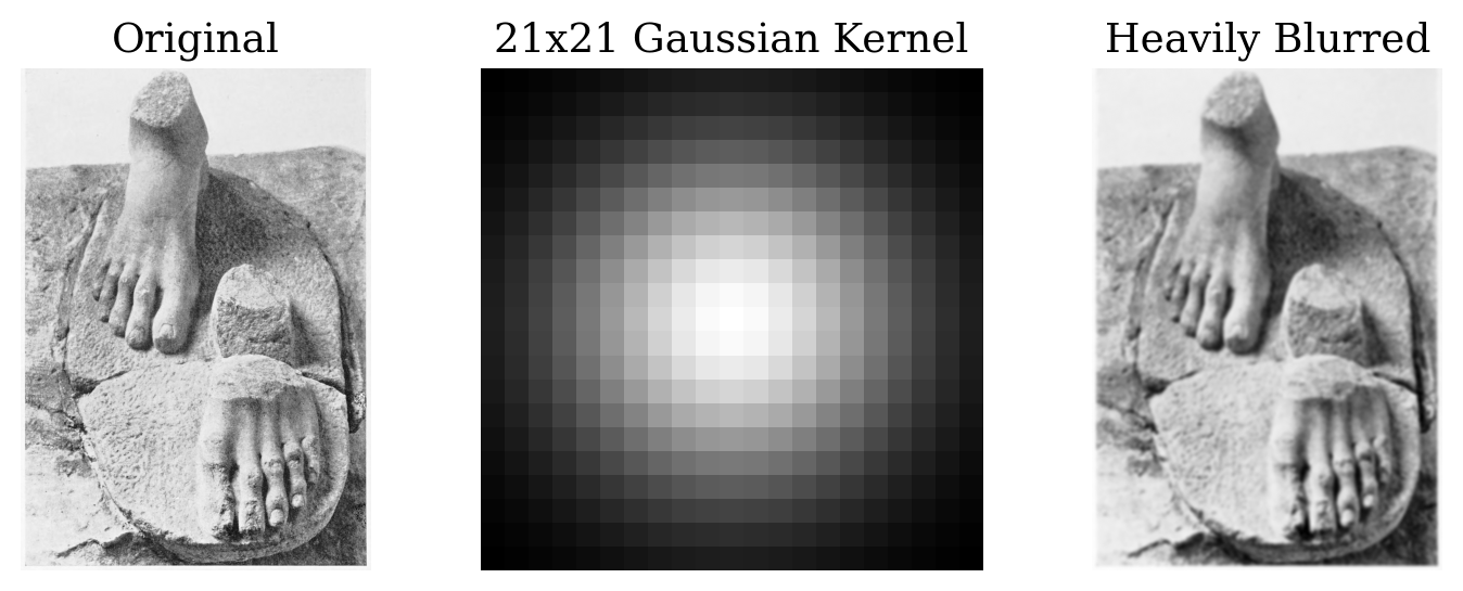
Below is a kernel that preserves the input image as it is; it is also known as the identity kernel:
img = np.array(Image.open(img_path).convert('L'))

# Identity kernel (3x3)
kernel = np.zeros((3, 3))
kernel[1, 1] = 1

conv = convolve(img, kernel)
fig, ax = plt.subplots(1, 3, figsize=(8, 3))
ax[0].imshow(img, cmap='gray'); ax[0].set_title("Original"); ax[0].axis('off')
ax[1].imshow(kernel, cmap='gray', vmin=0, vmax=1); ax[1].set_title("Identity Kernel"); ax[1].axis('off')
ax[2].imshow(conv, cmap='gray'); ax[2].set_title("Convolved"); ax[2].axis('off')
plt.tight_layout(); plt.show()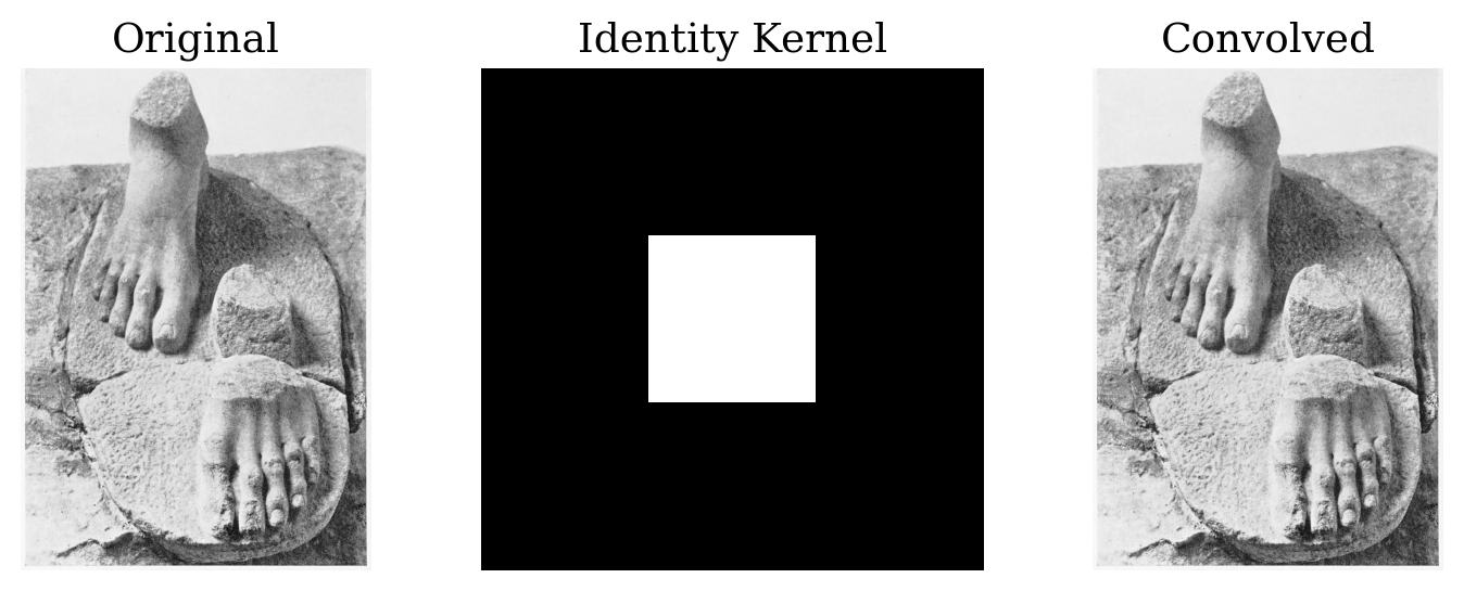
There is also a kernel that sharpens the images, known as the sharpening filter:
img = np.array(Image.open(img_path).convert('L'))

# Sharpen kernel
kernel = np.array([[ 0, -1,  0],
                   [-1,  5, -1],
                   [ 0, -1,  0]])

conv = convolve(img, kernel)
fig, ax = plt.subplots(1, 3, figsize=(8, 3))
ax[0].imshow(img, cmap='gray'); ax[0].set_title("Original"); ax[0].axis('off')
ax[1].imshow(kernel, cmap='gray'); ax[1].set_title("Sharpen Kernel"); ax[1].axis('off')
ax[2].imshow(conv, cmap='gray'); ax[2].set_title("Convolved"); ax[2].axis('off')
plt.tight_layout(); plt.show()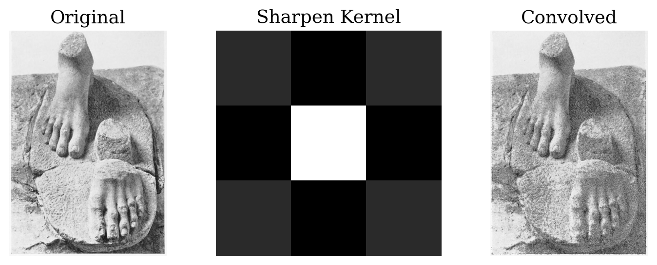
Other than sharpening, there is even a filter to emboss the image:
img = np.array(Image.open(img_path).convert('L'))

# Emboss kernel
kernel = np.array([[-2, -1, 0],
                   [-1,  1, 1],
                   [ 0,  1, 2]])

conv = convolve(img, kernel)
fig, ax = plt.subplots(1, 3, figsize=(8, 3))
ax[0].imshow(img, cmap='gray'); ax[0].set_title("Original"); ax[0].axis('off')
ax[1].imshow(kernel, cmap='gray'); ax[1].set_title("Emboss Kernel"); ax[1].axis('off')
ax[2].imshow(conv, cmap='gray'); ax[2].set_title("Convolved"); ax[2].axis('off')
plt.tight_layout(); plt.show()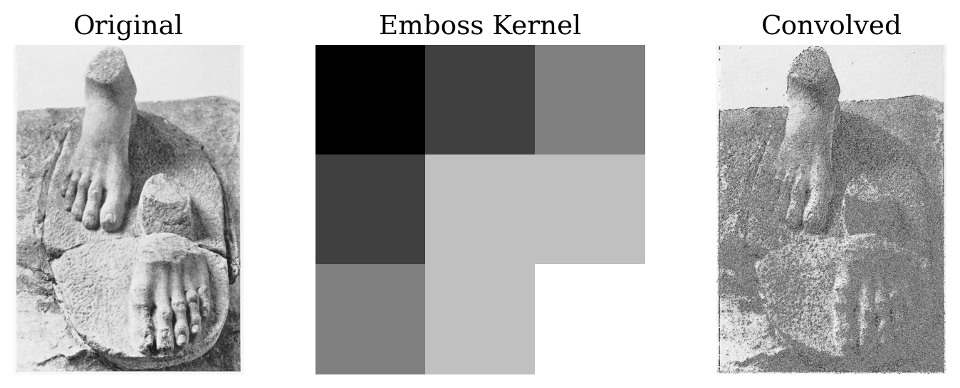
Other than only detecting vertical or horizontal edges, a filter named after Laplace was discovered to detect all edges:
img = np.array(Image.open(img_path).convert('L'))

laplacian = np.array([[0,-1,0],[-1,8,-1],[0,-1,0]])
edge = convolve(img, laplacian)

fig, ax = plt.subplots(1, 3, figsize=(8, 3))
ax[0].imshow(img, cmap='gray'); ax[0].set_title("Original"); ax[0].axis('off'
)
ax[1].imshow(laplacian, cmap='gray'); ax[1].set_title("Laplacian Kernel"); ax[1].axis('off')
ax[2].imshow(edge, cmap='gray'); ax[2].set_title("Edges"); ax[2].axis('off')
plt.tight_layout(); plt.show()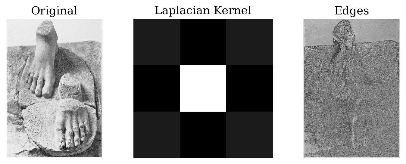
Over the years, people have discovered these tiny images or “kernels” or “filters”. In machine learning, we discover or learn these potentially useful filters directly from the data, rather than through mathematical derivation. In a word, machine learning can “learn” which filters would be useful for downstream tasks like classifying images or identifying things in an image.
# 1. Load a pretrained conv model (VGG16 without top)
model = VGG16(weights='imagenet', include_top=False)

# 2. Choose three conv layers: early, middle, late
early_layer = model.get_layer('block1_conv2')
mid_layer   = model.get_layer('block3_conv3')
late_layer  = model.get_layer('block5_conv3')

# 3. Extract one kernel from each layer
# Each kernel has shape (k, k, in_channels, out_channels)
kernel_early = early_layer.get_weights()[0][:, :, 0, 0]
kernel_mid   = mid_layer.get_weights()[0][:, :, 0, 0]
kernel_late  = late_layer.get_weights()[0][:, :, 0, 0]

# 4. Load and preprocess an image
def load_and_gray(path, target_size=(224,224)):
    img = keras_image.load_img(path, target_size=target_size)
    img_arr = keras_image.img_to_array(img)
    # convert to grayscale
    gray = cv2.cvtColor(img_arr.astype('uint8'), cv2.COLOR_RGB2GRAY)
    # normalize
    gray = gray.astype('float32') / 255.0
    return gray

gray = load_and_gray(img_path)

# 5. Convolve the image with each kernel
def apply_filter(img, kernel):
    # Flip kernel for convolution
    k = kernel.shape[0]
    # OpenCV uses correlation; flip kernel to perform convolution
    flipped = np.flipud(np.fliplr(kernel))
    filtered = cv2.filter2D(img, -1, flipped)
    return filtered

out_early = apply_filter(gray, kernel_early)
out_mid   = apply_filter(gray, kernel_mid)
out_late  = apply_filter(gray, kernel_late)

# 6. Visualize
plt.figure(figsize=(8, 8))

plt.subplot(2, 2, 1)
plt.title('Original Gray')
plt.imshow(gray, cmap='gray')
plt.axis('off')

plt.subplot(2, 2, 2)
plt.title('Early Layer Kernel')
plt.imshow(out_early, cmap='gray')
plt.axis('off')

plt.subplot(2, 2, 3)
plt.title('Mid Layer Kernel')
plt.imshow(out_mid, cmap='gray')
plt.axis('off')

plt.subplot(2, 2, 4)
plt.title('Late Layer Kernel')
plt.imshow(out_late, cmap='gray')
plt.axis('off')

plt.tight_layout()
plt.show()  # In Colab this will display inline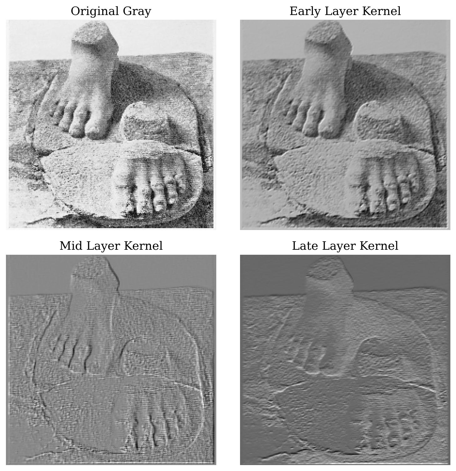
Different parts of the model highlight different things. The important thing to note is that no one wrote the filters themselves. The network learned that the features highlighted by these filters are useful. We simply wrote the learning algorithm, then the model learned from data by itself.
Typically, a model used for image classification can (on its own) learn filters to highlight things the model needs, such as edges and lines, and more importantly, in addition to these simple features, the model can learn filters to detect heads, eyes, ears, and other abstract concepts, and this is exactly how convolution makes it possible to detect, characterize, and categorize complex objects in complex images. In order to achieve these amazing features, we usually need to employ models such as Convolutional Neural Networks.
For the rest of the notebook, we will use a small selection of photographs from Richter’s Kouroi (1942), which contain frontal shots of Kouroi with a full torso and recognizable facial features. We have also prepared a labeled metadata that shows information about which group and era these Kouroi belong to and what materials they are made of. We can begin by looking at some basic information from the metadata:
# Read in the metadata CSV file
# Note that we are only going to investigate a subset of the full dataset
df = pd.read_csv('data/complete_sculpture_dataset_labeled.csv')

df = df.drop(columns = 'page')

print(df.head())
filename group era material
0 page188_img01_photo13.jpg SOUNION GROUP 615 - 590 BC Marble
1 page202_img01_photo3.jpg SOUNION GROUP 615 - 590 BC Marble
2 page202_img01_photo4.jpg SOUNION GROUP 615 - 590 BC Marble
3 page205_img01_photo4.jpg SOUNION GROUP 615 - 590 BC Marble
4 page211_img01_photo12.jpg SOUNION GROUP 615 - 590 BC Otherprint("Information of the dataset:")
print(f"Number of images: {df.shape[0]}")
print(f"Number of distinct eras: {df['era'].nunique()}")
print(f"Number of distinct materials: {df['material'].nunique()}")Information of the dataset:
Number of images: 62
Number of distinct eras: 7
Number of distinct materials: 3We can also see the distribution of each label by plotting histograms:
def bar_plot(df, column1, column2):
    # Calculate counts of each value in the specified columns
    label_counts1 = df[column1].value_counts()
    label_counts2 = df[column2].value_counts()

    # Create a figure with a fixed size
    fig, axes = plt.subplots(1, 2, figsize=(6, 3))

    # Plot the bar chart
    label_counts1.plot(kind='bar', ax=axes[0], color='steelblue')
    axes[0].set_title(f'Distribution of {column1.capitalize()}')
    axes[0].set_xlabel(column1.capitalize())
    axes[0].set_ylabel('Count')
    axes[0].tick_params(axis='x', rotation=90)
    label_counts2.plot(kind='bar', ax=axes[1], color='darkorange')
    axes[1].set_title(f'Distribution of {column2.capitalize()}')
    axes[1].set_xlabel(column2.capitalize())
    axes[1].set_ylabel('Count')
    axes[1].tick_params(axis='x', rotation=90)

    plt.tight_layout()
    plt.show()

# Plot the distribution of labels in the dataset
bar_plot(df, 'era', 'material')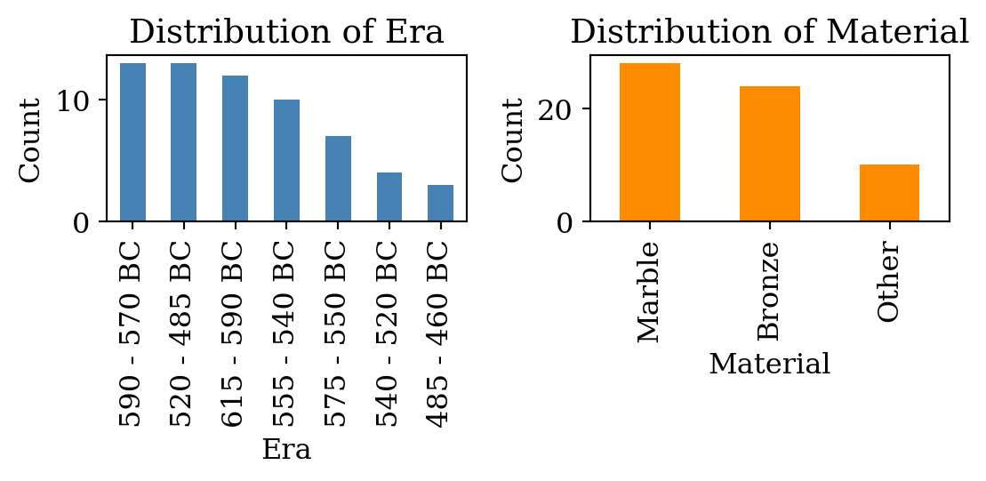
To get a direct idea of the general characteristics of this subset of photographs, we read the photographs from the image directory and show the first 4 images in this dataset.
# Read in the images as a list
data_dir = Path("data/richter_kouroi_complete_front_only")
image_paths = sorted(data_dir.glob("*.jpg"))

images = []
for p in image_paths:
    img = Image.open(p).convert("RGB")   # ensure 3‑channel
    img_arr = np.array(img)
    images.append(img_arr)

fig, axes = plt.subplots(1, 4, figsize=(6, 4))
for ax, img in zip(axes, images[:4]):
    ax.imshow(img)
    ax.axis("off")
plt.suptitle("First 4 images in the dataset")
plt.tight_layout()
plt.show()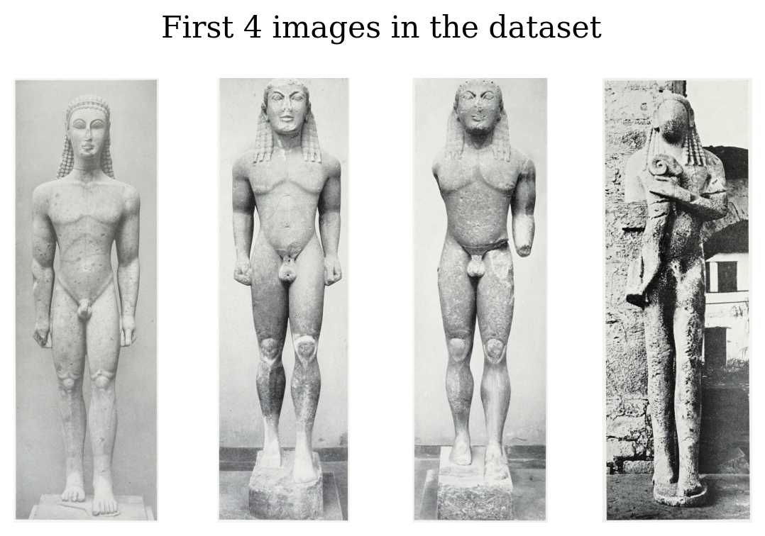
What we’ll do next is we will bring in ConvNeXt V2, it is a CNN model trained on millions of images based on ImageNet.
We’re sure everyone has used some Large Language Models (LLMs) and gotten a feel for how these models mimic the way humans think. This imitation of the human way of thinking comes from Artificial Neural Networks (ANN). Just as LLMs process and generate natural language, CNN models process visual images, examining the features in those images through convolutional layers and generating their own digital representations of the images.
Here, we will create a visualization that shows the early, middle, and late feature layers of the 4 images after convolution, what commonality and difference did you notice from the extracted features in these layers?
model = VGG16(weights='imagenet', include_top=False)

# Grab kernels from the first and last conv layers
early_layer = model.get_layer('block1_conv2')
mid_layer = model.get_layer('block3_conv3')
late_layer  = model.get_layer('block5_conv3')

# choose the (0,0) filter for each
kernel_early = early_layer.get_weights()[0][:, :, 0, 0]
kernel_mid  = mid_layer.get_weights()[0][:, :, 0, 0]
kernel_late  = late_layer.get_weights()[0][:, :, 0, 0]

# Convolution helper (flip kernel for true conv)
def apply_filter(img, kernel):
    flipped = np.flipud(np.fliplr(kernel))
    return cv2.filter2D(img, -1, flipped)

fig, axes = plt.subplots(3, 4, figsize=(8, 8))

for col, img in enumerate(images[:4]):
    gray = (
        cv2.cvtColor(img.astype('uint8'), cv2.COLOR_RGB2GRAY)
          .astype('float32') / 255.0
    )
    out_early = apply_filter(gray, kernel_early)
    out_early = (out_early - out_early.min()) / (out_early.max() - out_early.min())

    out_mid = apply_filter(gray, kernel_mid)
    out_mid = (out_mid - out_mid.min()) / (out_mid.max() - out_mid.min())

    out_late = apply_filter(gray, kernel_late)
    out_late = (out_late - out_late.min()) / (out_late.max() - out_late.min())

    # plot
    axes[0, col].imshow(out_early, cmap='gray')
    axes[0, col].set_title(f'Early Layer #{col+1}')
    axes[0, col].axis('off')

    axes[1, col].imshow(out_mid, cmap='gray')
    axes[1, col].set_title(f'Mid Layer #{col+1}')
    axes[1, col].axis('off')

    axes[2, col].imshow(out_late, cmap='gray')
    axes[2, col].set_title(f'Late Layer #{col+1}')
    axes[2, col].axis('off')

fig.suptitle('First, Middle vs. Last Conv Layer Responses', fontsize=16)
plt.tight_layout()
plt.show()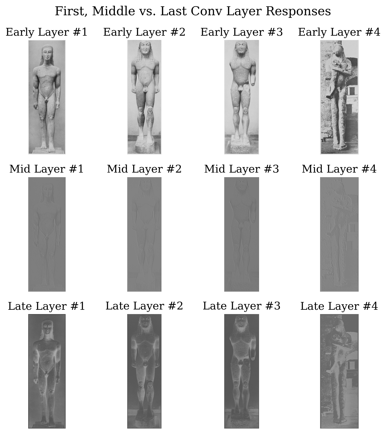
Image embedding is a process where images are transformed into numerical representations, specifically, lists of numbers that carry information about the images. While this sounds somewhat similar to the idea of visual words, they are not the same. Think of BoVW as counting how many times specific words appear in a book without caring about grammar or sentence structure– this can identify simple patterns, but cannot summarize the big picture of the book. Image embeddings, on the other hand, are like reading the entire book and summarizing its meaning in a well-crafted passage, they capture the bigger picture, context, and nuance.
We can build a vocabulary of visual words quite easily, but creating image embeddings usually requires using deep neural networks pretrained on millions of images. These networks process the entire image and learn hierarchical, abstract features that are more semantically meaningful.
Here, we will load the pre-trained ConvNeXt V2 model, pass the image folder to generate embeddings, and save the embeddings in a grid of numbers.
# Read in the pre-trained ConvNeXtV2 model
# Load the pre-trained ConvNeXtV2 model and image processor
processor = AutoImageProcessor.from_pretrained("facebook/convnextv2-base-22k-224")

# Move the model to the appropriate device (GPU or CPU)
device = torch.device("cuda" if torch.cuda.is_available() else "cpu")

model = ConvNextV2Model.from_pretrained("facebook/convnextv2-base-22k-224")

# Move the model to the appropriate device (GPU or CPU)
_ = model.to(device)

# Define the image directory for later use
image_directory = "data/richter_kouroi_complete_front_only"
Using a slow image processor as `use_fast` is unset and a slow processor was saved with this model. `use_fast=True` will be the default behavior in v4.52, even if the model was saved with a slow processor. This will result in minor differences in outputs. You'll still be able to use a slow processor with `use_fast=False`.# #| eval: false
# batch_size = 16
# embeddings = []
# valid_filenames = []
# filenames = df['filename'].tolist()
# for i in tqdm(range(0, len(filenames), batch_size), desc="Processing Images in Batches"):
# batch_filenames = filenames[i : i + batch_size]
# images = []
# for filename in batch_filenames:
# path = os.path.join(image_directory, filename)
# try:
# img = Image.open(path).convert("RGB")
# images.append(img)
# except FileNotFoundError:
# print(f"Missing: {path}")
# except Exception as e:
# print(f"Error with {filename}: {e}")
# if not images:
# continue
# # Prepare inputs
# inputs = processor(images=images, return_tensors="pt")
# pixel_values = inputs["pixel_values"].to(device)
# # Forward through feature extractor
# with torch.no_grad():
# outputs = model(pixel_values)
# # Global average pool
# if isinstance(outputs, torch.Tensor):
# hidden = outputs
# else:
# hidden = outputs.last_hidden_state
# batch_emb = hidden.mean(dim=(2, 3)).cpu().numpy()
# embeddings.extend(batch_emb)
# embeddings = np.stack(embeddings, axis=0)
# np.save('data/embeddings/convnextv2_image_embeddings.npy', embeddings)# Load embeddings from the saved file
embeddings = np.load('data/embeddings/convnextv2_image_embeddings.npy')
print(embeddings)
print(f"The embedding has {embeddings.shape[0]} rows and {embeddings.shape[1]} numbers each row.")[[-0.42546895 -4.1213956 -2.0160959 ... -2.990931 4.8743505
-0.30853495]
[ 0.5560602 -2.8647199 -2.922471 ... -1.7647432 4.883092
-0.54576755]
[-1.2865281 -1.4737651 -3.792193 ... 0.15527564 1.6415085
-1.8216568 ]
...
[-2.3245587 -3.1991036 -3.004582 ... -0.40073264 -0.21882926
0.5936357 ]
[-0.5283613 -4.433328 -3.7179348 ... -3.0150347 2.0326397
-1.6606904 ]
[ 0.31188568 -2.7383516 -3.1720133 ... -3.6925333 3.5139418
1.2292051 ]]
The embedding has 62 rows and 1024 numbers each row.We printed the embedded results above to see what they look like, and we also displayed the shape of the grid. As you can see, it contains 62 rows representing the 62 images in the dataset, and each row has 1024 numbers representing all the information extracted from each image. From now on, we will use this embedded data instead of the original image data.
1024 is way too many numbers for us to examine and understand with our brains. So, we use a technique called dimensionality reduction to squish the data down to just 2 or 3 dimensions, making it easy to visualize in 2D.
Principal Component Analysis (PCA) is one of such techniques, it is essentially finding the two or three major axes through our huge data along with which the data has the most variations. By PCA we decompose our data with 1024 dimensions (number of cells in each row) to 2 dimensions and represent each image as a point on our scatterplots. We then colour the data with “era” and “material” respectively.
Here, we will use plotly to create interactive visualizations, feel free to play with it and discuss patterns that you notice.
pio.renderers.default = "plotly_mimetype+notebook_connected"

# load metadata
df = pd.read_csv('data/complete_sculpture_dataset_labeled.csv')

# PCA to 2 components
pca = PCA(n_components=2)
pc2 = pca.fit_transform(embeddings)

# build DataFrame
pc_df = pd.DataFrame(pc2, columns=['PC1','PC2'])
pc_df['filename'] = df['filename'].values
pc_df['era'] = df['era'].values

# interactive scatter
fig = px.scatter(
        pc_df,
        x='PC1',
        y='PC2',
        color='era',
        hover_data=['filename'],
        title='Interactive PCA of Image Embeddings Colored by Era',
        width=700, height=500
    )

fig.show()pio.renderers.default = "plotly_mimetype+notebook_connected"
pc_df['material'] = df['material'].values
fig = px.scatter(
pc_df,
x='PC1',
y='PC2',
color='material',
hover_data=['filename'],
title='Interactive PCA of Image Embeddings Colored by Material',
width=700, height=500
)
fig.show()Discussion: Did you see any clear patterns of distributions by looking at the visualizations above? How can you interpret the results? What primary “features” do you think the PCA embedding captured in the first two dimensions?
Archaeological classification has always been an important issue in archaeology and artifact research. This problem is especially challenging when faced with a large amount of artifact data, or when faced with new artifacts with insufficient information. With the development of machine learning and image recognition technology, the use of computer technology to assist classification has become a trend in the new era of information archaeology. In this section, we would like to provide an example of classifying Kouroi by visual element for your reference.
In addition to observing how the labels are clustered based on the embeddings, we can train classifiers to categorize objects into appropriate labels based on the image embeddings directly. A traditional approach is through a technique called logistic regression.
X = embeddings
y1 = pc_df['era'].tolist()
y2 = pc_df['material'].tolist()

y1 = np.array(y1)
y2 = np.array(y2)
Note that here we use image embeddings and labels as training data and test data respectively, this is because we want to evaluate the effectiveness of the classifier when dealing with unseen data. After training the classifier for eras, we use it to predict the labels of the test data and compare the results with the real labels. The report is printed below:
# Perform the classification of eras
# Split the data into training and testing sets
X_train1, X_test1, y_train1, y_test1 = train_test_split(X, y1, test_size=0.25, random_state=42, stratify=y1)

# Create a logistic regression model
clf1 = LogisticRegression(max_iter=1000, random_state=42)

clf1.fit(X_train1, y_train1)

y_pred1 = clf1.predict(X_test1)

# Calculate classification metrics
classification_report1 = metrics.classification_report(y_test1, y_pred1, zero_division=0)

# Print the classification report
print("Classification Report for Eras:")
print(classification_report1)
Classification Report for Eras:
precision recall f1-score support
485 - 460 BC 0.00 0.00 0.00 1
520 - 485 BC 0.40 0.67 0.50 3
540 - 520 BC 0.00 0.00 0.00 1
555 - 540 BC 0.33 0.33 0.33 3
575 - 550 BC 0.00 0.00 0.00 2
590 - 570 BC 0.00 0.00 0.00 3
615 - 590 BC 0.50 0.33 0.40 3
accuracy 0.25 16
macro avg 0.18 0.19 0.18 16
weighted avg 0.23 0.25 0.23 16
The key metric we especially care about here is the accuracy of our classifier, it is defined by
\[ \text{Accuracy} = \frac{\text{True Predictions}}{\text{True Predictions} + \text{False Predictions}} \]
It reflects the proportion of true predictions out of all predictions made using the classifier. However, as shown above in the report, the accuracy of predicting era based on image embedding is not satisfactory. Still, we can visualize the decision boundary of this classifier on our 2D PCA of image embeddings to see what went wrong:
# Prepare your 2D data + labels
X_pca = pc_df[['PC1','PC2']].values
y_era = pc_df['era'].values

# Encode eras as integers
le = LabelEncoder()
y_enc = le.fit_transform(y_era)

# Train the logistic on the encoded labels
clf_2d = LogisticRegression(max_iter=1000, random_state=42)
clf_2d.fit(X_pca, y_enc)

# Build a mesh grid over the plotting area
x_min, x_max = X_pca[:,0].min() - 1, X_pca[:,0].max() + 1
y_min, y_max = X_pca[:,1].min() - 1, X_pca[:,1].max() + 1
xx, yy = np.meshgrid(
    np.linspace(x_min, x_max, 300),
    np.linspace(y_min, y_max, 300)
)

# Predict integer labels on the mesh
Z = clf_2d.predict(np.c_[xx.ravel(), yy.ravel()]).reshape(xx.shape)

# Plot the decision boundary
plt.figure(figsize=(7,7))

# Number of classes
n_classes = len(le.classes_)

# Pick a sequential colormap name:
base_cmap_red = plt.cm.Reds
base_cmap_blue = plt.cm.Blues

# Sample 7 colors evenly from the light part of the cmap for regions
# and the dark part for points.
region_colors = base_cmap_red(np.linspace(0.1, 0.6, n_classes))
point_colors  = base_cmap_blue(np.linspace(0.1, 1.0, n_classes))

cmap_light = ListedColormap(region_colors)
cmap_bold  = ListedColormap(point_colors)

plt.contourf(xx, yy, Z, alpha=0.3, cmap=cmap_light)

# scatter original points, mapping back to string labels in the legend
for class_int, era_label in enumerate(le.classes_):
    mask = (y_enc == class_int)
    plt.scatter(
        X_pca[mask,0], X_pca[mask,1],
        color=cmap_bold(class_int),
        label=era_label,
        edgecolor='k', s=40
    )

plt.xlabel('PC1')
plt.ylabel('PC2')
plt.title('Logistic Decision Boundary on 2D PCA Embedding\n(colored by era)')
plt.legend(title='Era')
plt.xlim(x_min, x_max)
plt.ylim(y_min, y_max)
plt.grid(True)
plt.show()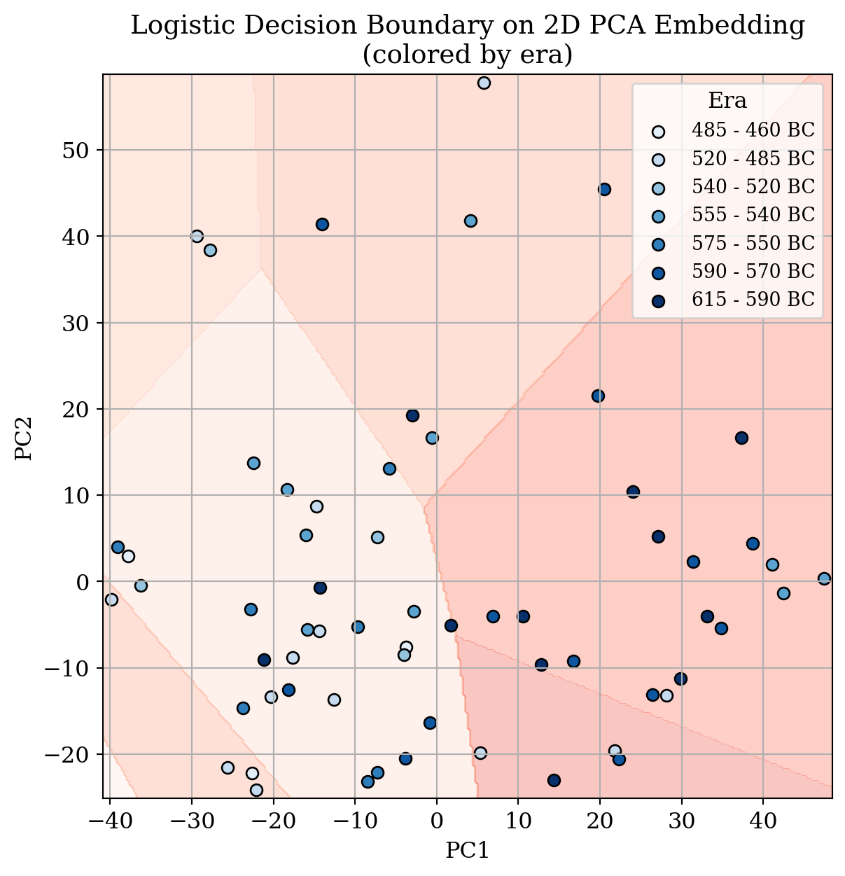
Discussion: What can you say about this decision boundary?
Similarly, we can use the same approach to classify material of Kouroi. We first perform a train-test split, then train the classifier, use the trained classifier to predict the labels of the test set, and print out the classification report for quality evaluation.
# Perform the classification of materials
# Split the data into training and testing sets
X_train2, X_test2, y_train2, y_test2 = train_test_split(X, y2, test_size=0.25, random_state=42, stratify=y2)

# Create a logistic regression model
clf2 = LogisticRegression(max_iter=1000, random_state=42)

clf2.fit(X_train2, y_train2)

y_pred2 = clf2.predict(X_test2)

# Calculate classification metrics
classification_report2 = metrics.classification_report(y_test2, y_pred2, zero_division=0)

# Print the classification report
print("Classification Report for Materials:")
print(classification_report2)
Classification Report for Materials:
precision recall f1-score support
Bronze 0.86 1.00 0.92 6
Marble 1.00 1.00 1.00 7
Other 1.00 0.67 0.80 3
accuracy 0.94 16
macro avg 0.95 0.89 0.91 16
weighted avg 0.95 0.94 0.93 16
As you can see, the accuracy is much higher now, but does that mean the classifier is good? You may have noticed that bronze and marble are classified almost perfectly, but other materials are not. This means that the classifier, while having a high accuracy, may have low precision or recall, as defined below:
We can also visualize the decision boundary on the 2D PCA of materials
# Prepare 2D data and labels
X_pca = pc_df[['PC1','PC2']].values
y_era = pc_df['material'].values

# Encode eras as integers
le = LabelEncoder()
y_enc = le.fit_transform(y_era)

# Train the logistic on the encoded labels
clf_2d = LogisticRegression(max_iter=1000, random_state=42)
clf_2d.fit(X_pca, y_enc)

# Build a mesh grid over the plotting area
x_min, x_max = X_pca[:,0].min() - 1, X_pca[:,0].max() + 1
y_min, y_max = X_pca[:,1].min() - 1, X_pca[:,1].max() + 1
xx, yy = np.meshgrid(
    np.linspace(x_min, x_max, 300),
    np.linspace(y_min, y_max, 300)
)

# Predict integer labels on the mesh
Z = clf_2d.predict(np.c_[xx.ravel(), yy.ravel()]).reshape(xx.shape)

# Plot the decision boundary
plt.figure(figsize=(7,7))

# light colors for regions
cmap_light = ListedColormap(['#FFCCCC','#CCFFCC','#CCCCFF','#FFE5CC','#E5CCFF'][:len(le.classes_)])
# bold colors for points
cmap_bold  = ListedColormap(['#FF0000','#00AA00','#0000FF','#FF8000','#8000FF'][:len(le.classes_)])

plt.contourf(xx, yy, Z, alpha=0.3, cmap=cmap_light)

# Scatter original points, mapping back to string labels in the legend
for class_int, era_label in enumerate(le.classes_):
    mask = (y_enc == class_int)
    plt.scatter(
        X_pca[mask,0], X_pca[mask,1],
        color=cmap_bold(class_int),
        label=era_label,
        edgecolor='k', s=40
    )

plt.xlabel('PC1')
plt.ylabel('PC2')
plt.title('Logistic Decision Boundary on 2D PCA Embedding\n(colored by material)')
plt.legend(title='Material')
plt.xlim(x_min, x_max)
plt.ylim(y_min, y_max)
plt.grid(True)
plt.show()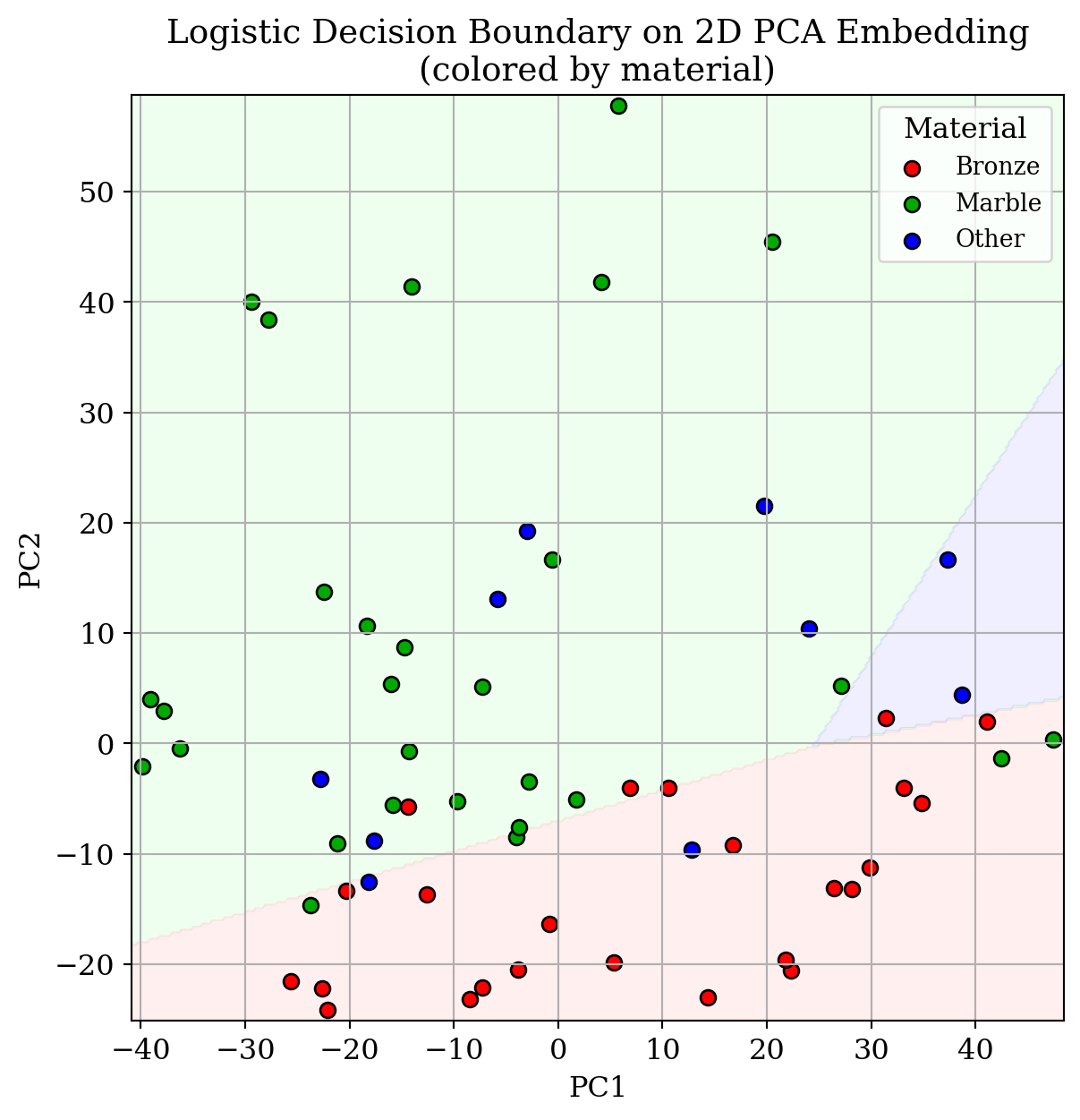
Discussion: Now, going back to the classification reports shown above, do you think the classifier trained on era is a good chronological classifier? What about materials?
The last classifier we’re going to visit today is a neural network classifier, using a Multi-layer Perceptron (MLP) network architecture, which means we’re going to add a classification layer to the ConvNeXt V2 model to classify the material. All the model does here is act as a backbone to observe and extract features of interest in the input image. The MLP process, on the other hand, can be visualized as a number of experts examining different features on an image, then discussing them with each other, and finally voting to reach a final conclusion.
We begin by creating the data loader and load the Kouroi data directly from the folder:
# Map the materials to integers
MAT2IDX = {
    'Marble': 0,
    'Bronze': 1,
    'Other': 2
}

# Create a custom dataset class for the Kouroi dataset
class KouroiDataset(Dataset):
    def __init__(self, df, img_dir, processor, mat2idx):
        self.df = df
        self.img_dir = image_directory
        self.processor = processor
        self.mat2idx = MAT2IDX

    def __len__(self):
        return len(self.df)

    def __getitem__(self, idx):
        row = self.df.iloc[idx]
        img = Image.open(os.path.join(self.img_dir, row.filename)).convert("RGB")

        inputs = self.processor(images=img, return_tensors="pt")

        for k,v in inputs.items():
            inputs[k] = v.squeeze(0)
        label = self.mat2idx[row.material]
return inputs, label# Train-test split
train_df, test_df = train_test_split(
df,
test_size=0.25, # 25% held out for testing
stratify=df["material"], # preserve class proportions
random_state=42
)
# Initialize the dataset and dataloader
train_ds = KouroiDataset(
df=train_df,
img_dir=image_directory,
processor=processor,
mat2idx=MAT2IDX
)
test_ds = KouroiDataset(
df=test_df,
img_dir=image_directory,
processor=processor,
mat2idx=MAT2IDX
)
train_loader = DataLoader(train_ds, batch_size=32, shuffle=True)
test_loader = DataLoader(test_ds, batch_size=32, shuffle=False)As mentioned above, here we freeze the model so that training does not change the way it understands the input image, but we are going to add a new classification layer on top of the network so that it can now use the additional knowledge about Kouroi for classification.
# Build the model with convnextv2 as the backbone and a linear layer for classification
class Classifier(nn.Module):
    def __init__(self, backbone_name, num_classes):
        super().__init__()
        # Load the ConvNeXtV2 backbone correctly and freeze it
        self.backbone = ConvNextV2Model.from_pretrained(
            backbone_name,
            output_hidden_states=False,
            output_attentions=False
        )
        for p in self.backbone.parameters():
            p.requires_grad = False

        embed_dim = self.backbone.config.hidden_sizes[-1]

        # Build a simple 2-layer MLP head
        self.head = nn.Sequential(
            nn.Linear(embed_dim, embed_dim // 2),
            nn.ReLU(inplace=True),
            nn.Dropout(0.2),
            nn.Linear(embed_dim // 2, num_classes)
        )

    def forward(self, pixel_values):
        # Forward through the frozen backbone
        outputs = self.backbone(pixel_values=pixel_values)
        x = outputs.pooler_output

        # Classification head
        logits = self.head(x)
        return logits

# Instantiate and move to device
model = Classifier(
    backbone_name="facebook/convnextv2-base-22k-224",
    num_classes=len(MAT2IDX)
).to(device)
Here, after setting up the new model, we will define the training loop and train the model. Please note that this process may take some time, especially when running on devices without a GPU. This also suggests that the high computational power requirement is a drawback when using CNNs for classification.
# #| eval: false
# # Set up the loss function and optimizer
# criterion = nn.CrossEntropyLoss()
# optimizer = optim.Adam(model.head.parameters(), lr=1e-4, weight_decay=0.01)
# epochs = 20

# for epoch in range(1, epochs+1):
#     model.train()
#     total_loss = 0
#     for batch in tqdm(train_loader, desc=f"Epoch {epoch}/{epochs}"):
#         inputs, labels = batch
#         # move to device
#         inputs = {k:v.to(device) for k,v in inputs.items()}
#         labels = labels.to(device)

#         optimizer.zero_grad()
#         logits = model(**inputs)
#         loss   = criterion(logits, labels)
#         loss.backward()
#         optimizer.step()

#         total_loss += loss.item() * labels.size(0)

#     avg_loss = total_loss / len(train_ds)
#     print(f" Epoch {epoch} avg loss: {avg_loss:.4f}")

# torch.save(model.state_dict(), "data/models/mlp_model.pth")
After training, we set the model to evaluation mode and assessed the classification quality by printing the confusion matrix and classification report. It is clear that the accuracy does improve with the MLP architecture. However, we still lacked samples of materials other than bronze and marble, which undoubtedly harmed the quality of our training.
# load the trained model
model.load_state_dict(torch.load("data/models/mlp_model.pth"))
model.to(device)  # move to the right device

# Run one pass over your data in eval mode
model.eval()

all_preds, all_labels = [], []
with torch.no_grad():
    for inputs, labels in test_loader:
        if inputs is None: continue
        inputs = {k:v.to(device) for k,v in inputs.items()}
        logits = model(**inputs)
        all_preds.extend(logits.argmax(dim=1).cpu().numpy())
        all_labels.extend(labels.numpy())

# Print the classification report
from sklearn.metrics import classification_report
report = classification_report(all_labels, all_preds, target_names=list(MAT2IDX.keys()), zero_division=0)
print("Classification Report for Materials:")
print(report)
Classification Report for Materials:
precision recall f1-score support
Marble 1.00 1.00 1.00 7
Bronze 0.75 1.00 0.86 6
Other 1.00 0.33 0.50 3
accuracy 0.88 16
macro avg 0.92 0.78 0.79 16
weighted avg 0.91 0.88 0.85 16
Discussion: What difference did you notice in the result? Does this mean that MLP is not applicable to classifying materials?
While the MLP classifier via CNN has advantages in dealing with more complex data structures (especially high-dimension nonlinear data), we note that it has two serious drawbacks: 1. it is more susceptible to the randomness of the training-testing split, with greater model variability; and 2. it is more susceptible to overfitting, whereas logistic regression is more susceptible to underfitting (for more detailed information on discussion of these concepts can be found in Appendix B). This tells us that no one model is perfect for all situations. We must remain cautious in our choice of models.
Now, let’s imagine a scenario where we find a new Kouros, but we are not sure what it is made of, and we want to use our trained classifier to classify it based on its image features.
# Define a new image to compare with the existing ones
new_artifact_path = 'data/example_images/NAMA_3938_Aristodikos_Kouros.jpeg'
new_artifact_label = 'A Kouros from Athens' # Suppose this is a new artifact we just discovered

art_new = cv2.imread(new_artifact_path, cv2.IMREAD_GRAYSCALE)

# Show the new image
plt.figure(figsize=(6, 6))
plt.imshow(art_new, cmap='gray')
plt.title(f"{new_artifact_label}")
plt.axis('off')
plt.show()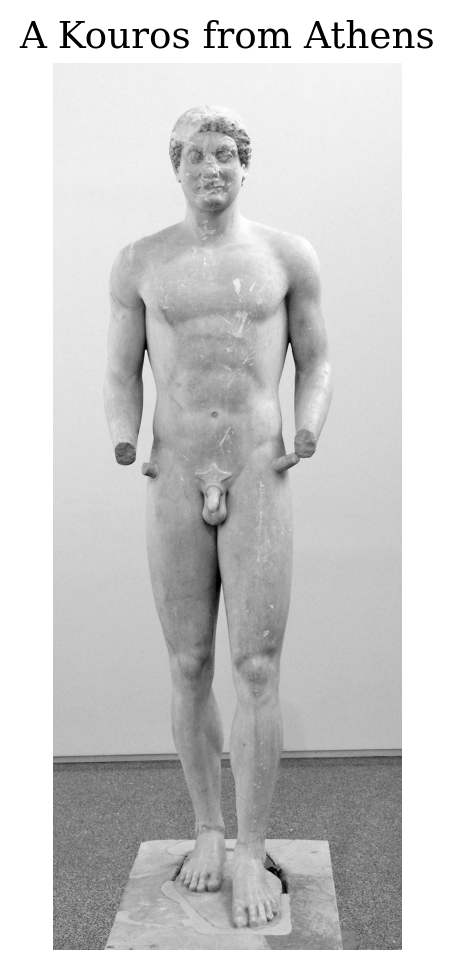
Discussion: Looking at this photo, how would you classify the era and material of this Kouros?
We pass it into our trained logistic regression classifier and see how would its era be classified:
# reload the processor and the model
processor = AutoImageProcessor.from_pretrained("facebook/convnextv2-base-22k-224")

model = ConvNextV2Model.from_pretrained("facebook/convnextv2-base-22k-224")

# Open as new img
img_new = Image.open(new_artifact_path).convert("RGB")

inputs = processor(images=img_new, return_tensors="pt")
pixel_values = inputs["pixel_values"].to(device)

# Forward through feature extractor
with torch.no_grad():
    outputs = model(pixel_values)

# Global average pool
if isinstance(outputs, torch.Tensor):
    hidden = outputs
else:
    hidden = outputs.last_hidden_state

emb_new = hidden.mean(dim=(2, 3)).cpu().numpy()


pred_era = clf1.predict(emb_new)[0]

print("Predicted Era:", pred_era)
Predicted Era: 540 - 520 BCWe then pass it into our trained CNN classifier and see how its material would be classified:
# reload the model
model = Classifier(
    backbone_name="facebook/convnextv2-base-22k-224",
    num_classes=len(MAT2IDX)
).to(device)
model.load_state_dict(torch.load("data/models/mlp_model.pth"))
model.to(device)

# Resize the model to an appropriate size
preprocess = transforms.Compose([
    transforms.Resize(256),
    transforms.CenterCrop(224),
    transforms.ToTensor(),
    transforms.Normalize(
        mean=[0.485, 0.456, 0.406],
        std= [0.229, 0.224, 0.225]
    ),
])

idx2mat = {idx: mat for mat, idx in MAT2IDX.items()}

def predict_image(image_path, model, device):
    # Load
    img = Image.open(image_path).convert("RGB")
    # Preprocess
    x = preprocess(img)
    x = x.unsqueeze(0).to(device)
    # Inference
    model.eval()
    with torch.no_grad():
        logits = model(**{"pixel_values": x}
                       if isinstance(x, torch.Tensor) else x)
        pred_idx = logits.argmax(dim=1).item()

    return idx2mat[pred_idx]

model.to(device)

predicted_material = predict_image(new_artifact_path, model, device)
print("Predicted Material:", predicted_material)
Predicted Material: MarbleDiscussion: Do you think the predictions made above are correct? What is your evidence?
What we didn’t really include here are the more advanced applications of fine-tuning. Fine-tuning refers to the process of taking a pre-trained model (like ConvNeXt V2) and continuing its training on your specific dataset, allowing the model to adapt its learned features to better suit your task. We did not cover fine-tuning here because it requires more computational resources, careful hyperparameter tuning, and a larger dataset to avoid overfitting. Additionally, fine-tuning can be time-consuming and is often not practical in an introductory or resource-limited setting.
However, fine-tuning has the potential to significantly improve classification quality, especially for irregular data. By allowing the model to update its internal representations based on the unique characteristics of your images, it can learn more relevant features for distinguishing between subtle differences in style, era, or material. For research or production applications with sufficient data and compute, fine-tuning is a powerful next step to achieve higher accuracy and more robust results.
Through this notebook, you’ve taken a journey with the example of Richter’s Kouroi from the basics of how computers “see” images to advanced techniques for analyzing and classifying images. You’ve explored how simple pixel values can be transformed into powerful representations using convolution, image embeddings, and neural networks. Along the way, you learned to visualize, cluster, and classify artworks…… these are all skills that are at the heart of modern computer vision.
Remember, the tools and concepts you’ve practiced here are not just limited to art history or archaeology: they are widely used in fields ranging from medicine to astronomy, and beyond. As you continue your studies, keep experimenting, stay curious, and don’t be afraid to explore new datasets or try more advanced models. The intersection of technology and the humanities is full of exciting possibilities, and your creativity is the key to unlocking them.
Congratulations on completing this exploration, and we hope you feel inspired to keep learning and discovering the field of Machine Learning!
.pdf FilesThis part provides a brief overview of how the data was collected and preprocessed for the analysis, typically how we cropped the images and prepared the metadata.
We used the following python script to convert a scanned pdf of Richter (1942) to image files in .jpg format.
import fitz

# Change the filename here if you want to reuse the script for your own project
doc = fitz.open("kouroiarchaicgre0000rich_1.pdf")

import os
out_dir = "extracted_images"
os.makedirs(out_dir, exist_ok=True)

# Iterate pages
for page_index in range(len(doc)):
    page = doc[page_index]
    image_list = page.get_images(full=True)  # get all images on this page

    # Skip pages without images
    if not image_list:
        continue

    # Extract each image
    for img_index, img_info in enumerate(image_list, start=1):
        xref = img_info[0]
        base_image = doc.extract_image(xref)
        image_bytes = base_image["image"]
        image_ext   = base_image["ext"]

        # Write to file
        out_path = os.path.join(
            out_dir,
            f"page{page_index+1:03d}_img{img_index:02d}.{image_ext}"
        )
        with open(out_path, "wb") as f:
            f.write(image_bytes)

print(f"Saved all images to {out_dir}")
The following script cropped the photos by applying convolution.
import cv2
import glob
import os

# Folder containing your page images
input_folder = "extracted_images"
output_folder = "cropped_photos"
os.makedirs(output_folder, exist_ok=True)

def extract_photos_from_page(image_path, min_area=5000):
    img = cv2.imread(image_path)
    gray = cv2.cvtColor(img, cv2.COLOR_BGR2GRAY)
    # Blur and threshold to get binary image
    blurred = cv2.GaussianBlur(gray, (5, 5), 0)
    _, thresh = cv2.threshold(blurred, 200, 255, cv2.THRESH_BINARY_INV)

    # Dilate to merge photo regions
    kernel = cv2.getStructuringElement(cv2.MORPH_RECT, (15, 15))
    dilated = cv2.dilate(thresh, kernel, iterations=2)

    # Find contours
    contours, _ = cv2.findContours(dilated, cv2.RETR_EXTERNAL, cv2.CHAIN_APPROX_SIMPLE)

    crops = []
    for cnt in contours:
        x, y, w, h = cv2.boundingRect(cnt)
        area = w * h
        # Filter by area to remove small artifacts
        if area > min_area:
            crop = img[y:y+h, x:x+w]
            crops.append((crop, (x, y, w, h)))
    return crops

# Process all pages
for img_path in glob.glob(os.path.join(input_folder, "*.*")):
    base = os.path.splitext(os.path.basename(img_path))[0]
    photos = extract_photos_from_page(img_path)
    for idx, (crop, (x, y, w, h)) in enumerate(photos, start=1):
        out_file = os.path.join(output_folder, f"{base}_photo{idx}.jpg")
        cv2.imwrite(out_file, crop)

print(f"Saved all images at {output_folder}")
The following script employed tesseract OCR engine to detect pure text images and filter out photos of Kouros. You may want to visit the GitHub repository https://github.com/tesseract-ocr/tesseract to see how to install and setup appropriately.
import os
import shutil
from PIL import Image
import pytesseract
# Ensure you have Tesseract installed and pytesseract configured correctly.
# On Windows, you might need:
# pytesseract.pytesseract.tesseract_cmd = r'C:\Program Files\Tesseract-OCR\tesseract.exe'

# Folders
input_folder = "cropped_photos"
text_folder = "text_crops"
photo_folder = "filtered_photos"
os.makedirs(text_folder, exist_ok=True)
os.makedirs(photo_folder, exist_ok=True)

# Threshold for text length to consider as "text-only"
# You can also adjust this threshold based on your specific needs.
TEXT_CHAR_THRESHOLD = 2 # Be careful with this threshold, do remember to check the results manually


for filename in os.listdir(input_folder):
    path = os.path.join(input_folder, filename)
    img = Image.open(path)

    # Perform OCR to extract text
    extracted_text = pytesseract.image_to_string(img)

    # Classify based on length of extracted text
    if len(extracted_text.strip()) >= TEXT_CHAR_THRESHOLD:
        dest = os.path.join(text_folder, filename)
    else:
        dest = os.path.join(photo_folder, filename)

    shutil.move(path, dest)
    print(f"Moved {filename} -> {os.path.basename(dest)}")

print("Filtering complete")
This script creates a .csv file for manual labelling.
import os, re
import pandas as pd

# Scan your filtered_photos folder
records = []

# Updated regex to match "page<number>_img<number>_photo<number>.<ext>"
pattern = re.compile(r"page(\d+)_img\d+_photo(\d+)\.(?:png|jpe?g)", re.IGNORECASE)

for fn in os.listdir("richter_kouroi_head_front_only"):
    m = pattern.match(fn)
    if not m:
        continue
    page = int(m.group(1))
    photo_idx = int(m.group(2))
    records.append({
        "filename": fn,
        "page": page,
        "group": "",    # blank for manual entry
        "era": "",  # blank for manual entry
        "material": ""  # blank for manual entry
    })

# Build DataFrame
df = pd.DataFrame(records)

df.sort_values(["page", "filename"], inplace=True)

# Save out to CSV for manual labeling
df.to_csv("label_template.csv", index=False)
You can try out the scripts with your interested pdf files yourself by running them in a python environment.
In the context of machine learning, two common pitfalls are underfitting and overfitting.
Underfitting occurs when a model is too simple to capture the underlying patterns in the data, resulting in poor performance on both the training and test sets. This is often seen when using models like logistic regression on complex, non-linear datasets, as shown in the left panel above, where the decision boundary fails to separate the classes effectively. On the other hand, overfitting happens when a model is excessively complex, such as a deep neural network with many layers, and learns not only the true patterns but also the noise in the training data. This leads to excellent performance on the training set but poor generalization to new, unseen data, as illustrated in the right panel where the decision boundary is overly intricate.
Let’s examine the two problems with a simulated two-class data:
# Generate a simulated two-class data
X, y = make_moons(n_samples=500, noise=0.40, random_state=0)

# Visualize the simulated data
plt.figure(figsize=(6, 4))
plt.scatter(X[:, 0], X[:, 1], c=y, cmap='coolwarm', edgecolor='k')
plt.xlabel('Feature 1')
plt.ylabel('Feature 2')
plt.title('Simulated Two-Class Data')
plt.show()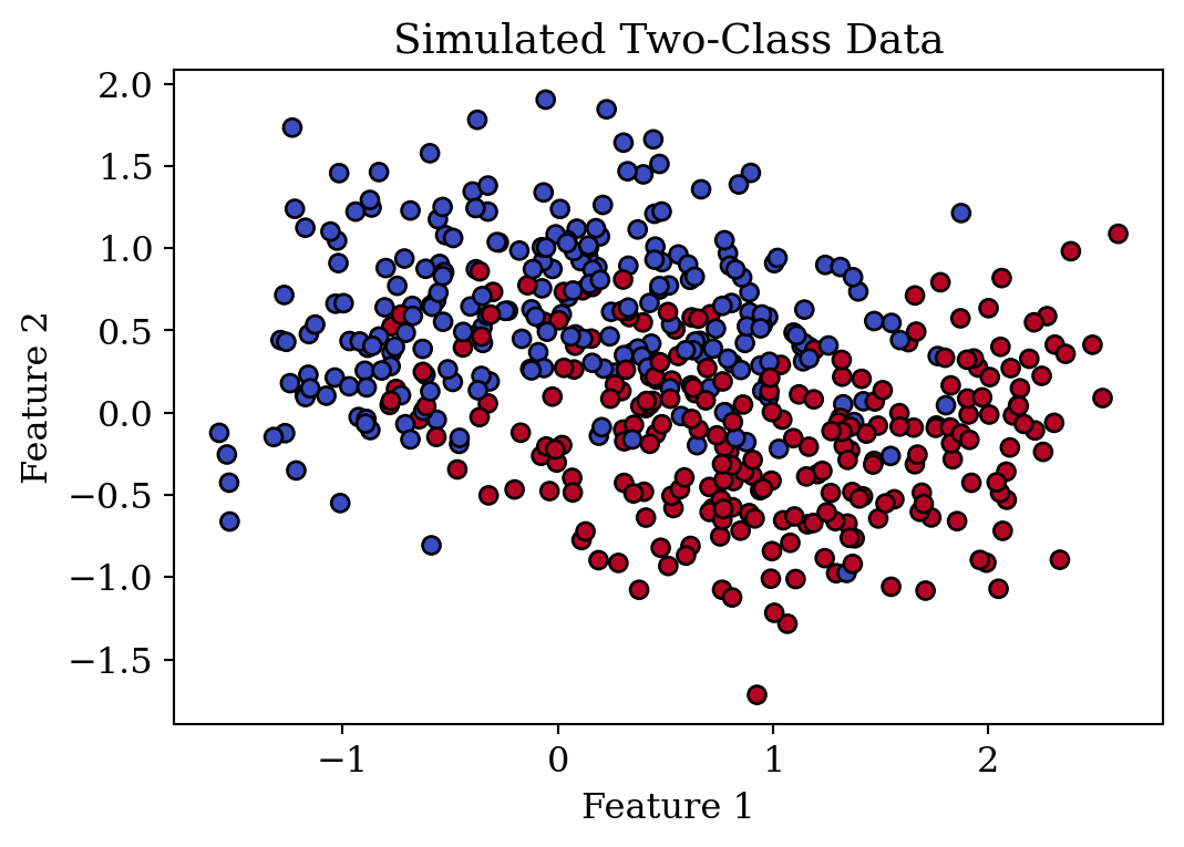
We can clearly see that the data is very non-linear, which gives us a hint that the right model should be able to account for non-linear relationships. However, for demonstration purposes, I will be using logistic regression to generate an underfitting classifier; and while MLP is suitable for use here, I will let it generate an overfitting classifier by significantly oversizing the neurons and iterations.
X_train, X_test, y_train, y_test = train_test_split(
    X, y, test_size=0.25, random_state=1
)
under = LogisticRegression()

over  = MLPClassifier(hidden_layer_sizes=(200,200,200),
                      max_iter=2000,
                      random_state=1)

# Train both models
under.fit(X_train, y_train)
over.fit(X_train, y_train)
MLPClassifier(hidden_layer_sizes=(200, 200, 200), max_iter=2000, random_state=1)In a Jupyter environment, please rerun this cell to show the HTML representation or trust the notebook.
MLPClassifier(hidden_layer_sizes=(200, 200, 200), max_iter=2000, random_state=1)
Then, we get the decision boundaries of the two classifiers and visualize them with the test data, what do you find about their accuracy?
# Build grid
x_min, x_max = X[:,0].min() - .5, X[:,0].max() + .5
y_min, y_max = X[:,1].min() - .5, X[:,1].max() + .5
xx, yy = np.meshgrid(
    np.linspace(x_min, x_max, 300),
    np.linspace(y_min, y_max, 300)
)
grid = np.c_[xx.ravel(), yy.ravel()]

# Get decision boundary
Zu = under.predict_proba(grid)[:,1].reshape(xx.shape)
Zo = over.predict_proba(grid)[:,1].reshape(xx.shape)

# Plot side by side
fig, (ax1, ax2) = plt.subplots(1, 2, figsize=(8,4))

for ax, Z, title in [
    (ax1, Zu, 'Extreme Underfit'),
    (ax2, Zo, 'Extreme Overfit')
]:
    ax.contourf(xx, yy, Z>0.5, alpha=0.3)
    # draw precise decision boundary P=0.5
    ax.contour(   xx, yy, Z, levels=[0.5], colors='k', linewidths=1.5)

    ax.scatter(X_test[:,0], X_test[:,1], c=y_test, edgecolor='k')
    ax.set_title(title)
    ax.set_xlabel('Feature 1')
    ax.set_ylabel('Feature 2')

fig.suptitle('Underfitting vs. Overfitting in Classification', fontsize=16)
plt.tight_layout(rect=[0,0.03,1,0.95])
plt.show()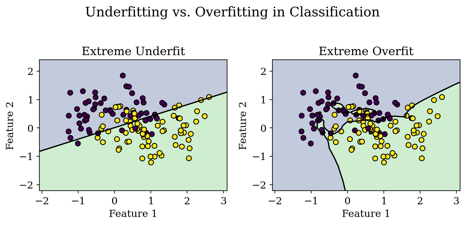
We can tell easily from the above visualization that both scenarios are harmful: underfitting prevents the model from making meaningful predictions, while overfitting results in unreliable predictions on real-world data. The example above also highlights the necessity to validate classifier quality using test data.
While underfitting and overfitting can seem scary, there are many tools that have been developed to address this issue. We can adjust the complexity of the model, use regularization techniques, collect more data, or employ cross-validation to find a balance that generalizes well to new examples. These are left for you to explore on your own.