import sqlite3
import pandas as pdBasic Querying
Python
SQL
joins
data engineering
The second notebook in the Data Engineering stream, and your first job as a data analyst: the research team needs one deliverable, a regional wage briefing. On the way there you learn the core of SQL inside a single SELECT: joins and why they change row counts, GROUP BY and HAVING, the NULLs (which nearly get you fired), CASE logic, and edit many plausible-looking wrong queries. It ends with a question this notebook’s tools cannot answer.
Outline
Prerequisites
- Notebook 1 of this stream: what a database and a DBMS are,
SELECT,WHERE,ORDER BY, and running SQL through%%sqlcells.
Learning Outcomes
By the end of this notebook you will be able to:
- Combine tables with inner and left joins, and predict how a join changes the number of rows.
- Summarize data with aggregates and
GROUP BY, and state the logical order in which SQL evaluates a query, including whereHAVINGfits. - Explain NULL and three-valued logic: why
= NULLfinds nothing, and how NULLs silently shape counts and averages. - Build categories inside a query with
CASE. - Spot and fix plausible-looking wrong queries.
1. Where we are in the stream
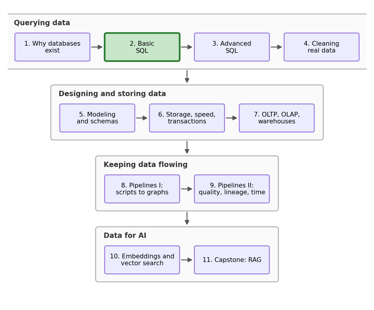
Notebook 1 ended with us looking at one table at a time. This notebook is the core of SQL: everything an analyst does most days, and everything a screening interview asks about, built from a single SELECT. SQL is the language the world of data speaks, and it is far easier to learn than Python, R, C++ or any other programming language. It is truly intuitive, and with a little effort you will understand all of it. But we can make this effort fun (hopefully at least a little).
So instead of learning it like a manual, we will learn it on the job. You have just joined the survey’s research team as its data analyst (congratulations!!!), and the team is writing a short report on Canadian wages. One deliverable is yours: a single table, wages by region, full-time workers only, with worker counts and union shares.
This is not a made-up type of table. Here is Statistics Canada’s version, wages and hours by union status, from the Labour Force Survey:
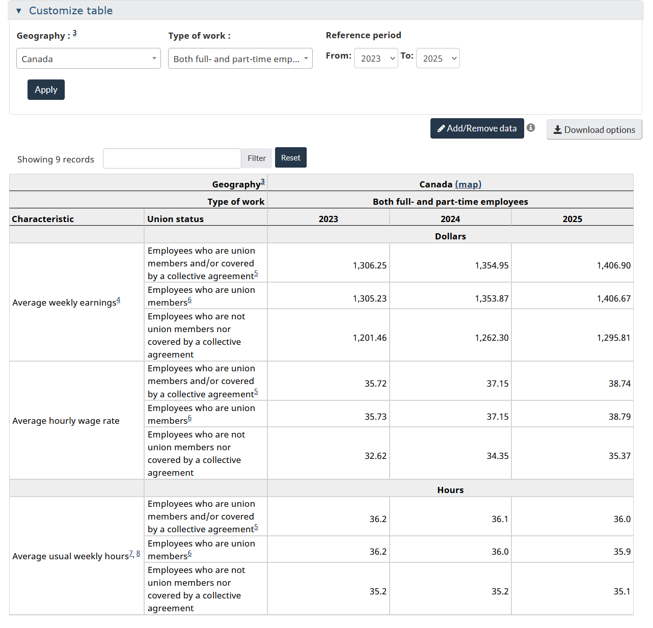
Along the way runs a wrong-query gallery: plausible-looking queries that do not do what their author wanted, sometimes with errors, but usually silently. Your colleagues will be submitting a few of these. Learning to catch them is a real skill.
2. One table becomes three
So far all of our data has lived in one table, and every question was answered by scanning that one table. This is the largest conceptual step from a standalone file (like a .csv) to a database.
A real database is almost never one big table. It is a collection of tables, where each table holds one kind of thing: one row per survey respondent, one row per province, one row per certification. The obvious question is why. Why not throw everything into a single wide table? Try it mentally with our data and it breaks in two different ways:
- Facts about provinces would repeat once per respondent. British Columbia’s minimum wage would be stored 353 times, once in every BC row, and in the next few years when the rate changes, you would need to update all 353 copies perfectly or the data breaks. Notebook 1 named this disease: redundancy.
- Certifications do not fit the survey’s shape at all. One respondent holds three certifications, another holds none. Do you add columns
certification_1,certification_2,certification_3, and break on the first person with four? Or repeat the person’s whole row once per certification, duplicating their wage and corrupting every average? Both options are bad, because “one row per person” is simply the wrong shape for facts that come in variable numbers per person.
The relational answer is to give each kind of thing its own table, store every fact only once, and connect the tables through shared columns. Here is what our database looks like from this notebook on, drawn with real rows from each table:
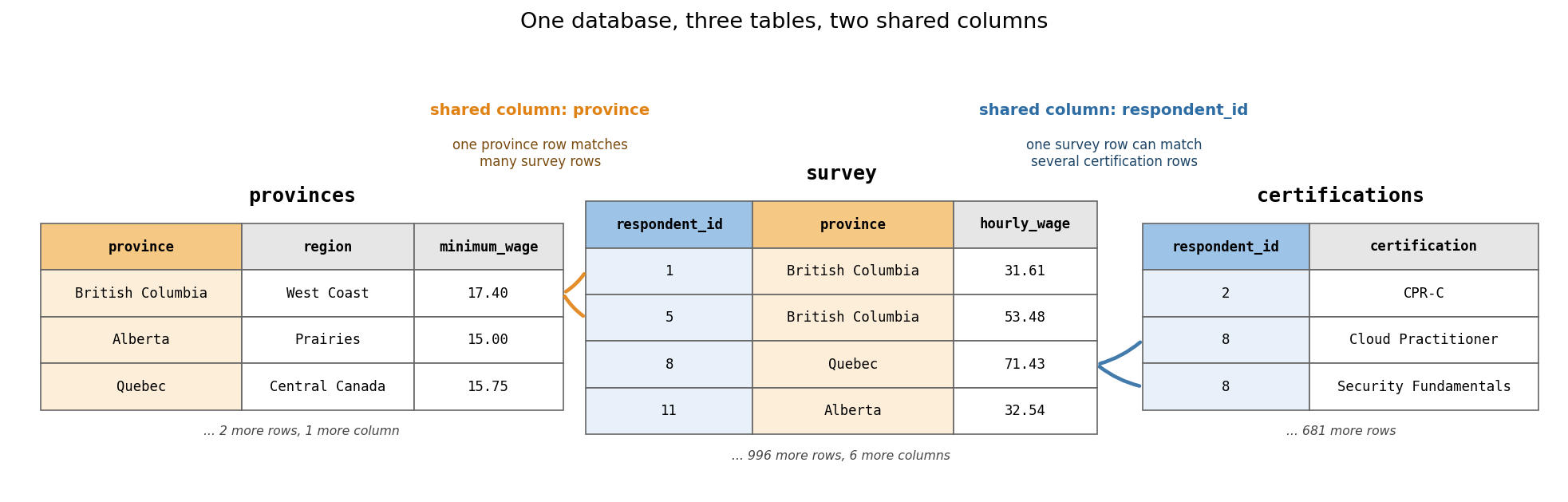
Read it row by row, following the arrows. Respondents 1 and 5 both live in British Columbia, so both of their rows match the same single provinces row: BC’s minimum wage of 17.40 is stored exactly once as well, whether 2 respondents point at it or all 353 who live there. On the other side, respondent 8 listed two certifications, so their one survey row matches two certifications rows. The shared columns doing the pointing, province on one side and respondent_id on the other, are called join keys, and section 4 is about the command that follows them.
First, the setup. We rebuild the database from the raw files so this notebook can be run alone without NB1:
provinces = pd.read_csv("datasets/provinces.csv")
certifications = pd.read_csv("datasets/certifications.csv")

conn = sqlite3.connect("datasets/wage_survey.db")
pd.read_csv("datasets/wage_survey.csv").to_sql("survey", conn, index=False, if_exists="replace")
provinces.to_sql("provinces", conn, index=False, if_exists="replace")
certifications.to_sql("certifications", conn, index=False, if_exists="replace")684The 684 that the cell reports is the row count of the last table written, certifications.
%load_ext sql
%config SqlMagic.autopandas = True
%config SqlMagic.displaycon = False
%config SqlMagic.feedback = 0
%sql sqlite:///datasets/wage_survey.db
Before querying anything, look at the two new datasets side by side:
print(provinces.to_string(index=False))
print()
print(certifications.head(6).to_string(index=False))
province region minimum_wage population
British Columbia West Coast 17.40 5719961
Alberta Prairies 15.00 4980659
Manitoba Prairies 15.80 1507330
Ontario Central Canada 17.20 16176977
Quebec Central Canada 15.75 9110616
respondent_id certification
2 CPR-C
4 First Aid Level 1
8 Cloud Practitioner
8 Security Fundamentals
10 First Aid Level 1
10 WHMISThe first table, provinces, is a lookup table (also called a reference table): one row per province. It has only five rows, one per province, and holds values associated with each province, nothing about any individual respondent. Unlike the survey from NB1, this data is real. The minimum wages are the true legal rates in April 2025, from the Government of Canada’s minimum wage database, and the populations are Statistics Canada’s estimates for April 1, 2025; the region grouping is ours. It fits our survey through the province column: every respondent’s province should have a row here. It also matters for the job: the briefing wants regions, and the survey does not have a region column. This little table is where regions live.
The second table, certifications, is a new module of our simulated survey: respondents listed the job certifications they hold, one row per certification held. What one row stands for is different again, a person-certificate pair rather than a person, which is why respondents 8 and 10 each appear twice in the first six rows (respondent 8 with certifications for Cloud Practitioner and Security Fundamentals). It fits our survey through respondent_id, it is important to note, not all respondents had certifications: 548 of our 1,000 respondents listed none and so have no rows here at all, while others have two or three. This module is simulated because it has to be: Statistics Canada publishes real survey microdata, but public files are anonymized before release, and the respondent identifiers that link tables together, the exact thing this section teaches, are among the first things anonymization removes.
This three-table setup is a miniature of every production database you will ever work with: a big table of people or events, lookup tables describing the categories they belong to, and detail tables holding the facts that come in variable numbers. The rest of the notebook is about asking questions across all three.
3. Sizing up the data
Rule one of reporting on data: profile it before you summarize it. Nobody should publish numbers from a table they have never actually looked at, so before the briefing gets its first draft, we look into the survey. The profiling workhorse is DISTINCT, which removes duplicates from the result, every unique entry exactly once, and so answers the question “what does this column actually contain?”
%%sql
SELECT DISTINCT province
FROM survey| province | |
|---|---|
| 0 | British Columbia |
| 1 | Ontario |
| 2 | Quebec |
| 3 | Manitoba |
| 4 | Alberta |
| 5 | Saskatchewan |
Six provinces, each exactly once. Notebook 1’s table of typical file failures had BC, B.C., bc, and Britsh Columbia all meaning one province; in a database with enforced categories, the same question is one keyword, and if the survey held even a single row with a new spelling, DISTINCT would expose it immediately.
4. Crossing tables: JOIN
The briefing wants wages by region. Wages live in survey, regions live in provinces, so we can’t use a single table to answer this question. Section 2 split our data apart and promised a command that connects it back together; this is JOIN, and it is the single most important idea in this notebook.
A join combines two tables by pairing up their rows wherever a matching rule holds. The rule almost always says that a shared column agrees on both sides, and that shared column is the join key from section 2’s diagram: province links the survey to provinces, and respondent_id links it to certifications. Use a JOIN whenever a question needs columns from more than one table, which in real work is most questions.
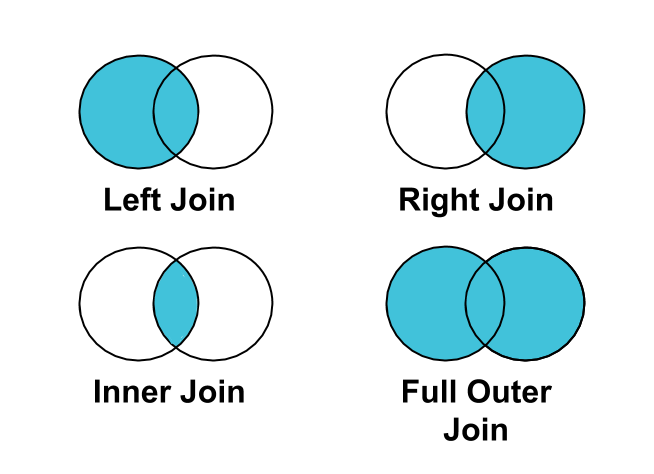
The classic picture of the join family looks like this, where each circle is a table and the shading marks which rows survive:
4.1 The inner join
The syntax has three new pieces:
FROM survey AS s JOIN provinces AS pnames both tables and gives each a short alias (sandp), so the rest of the query can refer to them without spelling the full names out.ON s.province = p.provinceis the matching rule: pair up rows where the provinces agree.s.provinceandp.provinceare qualified column names. Both tables have a column calledprovince, so every mention has to say whose it is, alias first, then a dot.
Predict first.
surveyhas 1,000 rows andprovinceshas 5. Before you run the next cell, commit to a number: how many rows will the join return?
%%sql
SELECT s.respondent_id, s.province, p.region, p.minimum_wage
FROM survey AS s
JOIN provinces AS p ON s.province = p.province| respondent_id | province | region | minimum_wage | |
|---|---|---|---|---|
| 0 | 1 | British Columbia | West Coast | 17.40 |
| 1 | 2 | Ontario | Central Canada | 17.20 |
| 2 | 3 | Quebec | Central Canada | 15.75 |
| 3 | 4 | Ontario | Central Canada | 17.20 |
| 4 | 5 | British Columbia | West Coast | 17.40 |
| ... | ... | ... | ... | ... |
| 949 | 996 | Ontario | Central Canada | 17.20 |
| 950 | 997 | Ontario | Central Canada | 17.20 |
| 951 | 998 | Ontario | Central Canada | 17.20 |
| 952 | 999 | Alberta | Prairies | 15.00 |
| 953 | 1000 | Quebec | Central Canada | 15.75 |
954 rows × 4 columns
Each result row is a survey row with its matching province facts attached. But read the output: 954 rows. It’s not 1,000 or 5, and if you predicted either, you have just learned the most useful lesson in this section. A plain JOIN (an inner join) keeps only the rows that find a match, and Saskatchewan’s 46 respondents found none, because the profile in section 3 counted six provinces and our lookup table holds five. They were dropped, and nothing warned us or printed an error. If your next step were “average wage by region”, those 46 people would not exist. This is a problem and your boss would not be happy.
4.2 The left join
A left join keeps every row of the left table (the one named in FROM), matched or not, and fills the right table’s columns with NULL where no match exists. Use it in two situations: when losing unmatched rows is unacceptable (like in this case where every respondent must count), and when the unmatched rows are themselves the thing you are hunting for, because a left join is how you find out which of your rows have no partner.
%%sql
SELECT s.respondent_id, s.province, p.region, p.minimum_wage
FROM survey AS s
LEFT JOIN provinces AS p ON s.province = p.province
ORDER BY p.region| respondent_id | province | region | minimum_wage | |
|---|---|---|---|---|
| 0 | 40 | Saskatchewan | None | NaN |
| 1 | 41 | Saskatchewan | None | NaN |
| 2 | 45 | Saskatchewan | None | NaN |
| 3 | 52 | Saskatchewan | None | NaN |
| 4 | 64 | Saskatchewan | None | NaN |
| ... | ... | ... | ... | ... |
| 995 | 968 | British Columbia | West Coast | 17.4 |
| 996 | 969 | British Columbia | West Coast | 17.4 |
| 997 | 989 | British Columbia | West Coast | 17.4 |
| 998 | 992 | British Columbia | West Coast | 17.4 |
| 999 | 995 | British Columbia | West Coast | 17.4 |
1000 rows × 4 columns
1,000 rows, nobody dropped, and the Saskatchewan respondents sit at the top of the sort with None and NaN where a region and minimum wage should be. Those empty cells are NULLs, and in section 6 they will come very close to ruining our briefing.
4.3 Joins that multiply
So far joins have shrunk our table or preserved it. They can also make it grow.
Predict first. Some respondents have no rows in
certifications, some have two or three. Will joining the survey to it return more or fewer than 1,000 rows?
%%sql
SELECT s.respondent_id, s.industry, s.hourly_wage, c.certification
FROM survey AS s
JOIN certifications AS c ON s.respondent_id = c.respondent_id| respondent_id | industry | hourly_wage | certification | |
|---|---|---|---|---|
| 0 | 2 | Health care | 49.16 | CPR-C |
| 1 | 4 | Education | 26.09 | First Aid Level 1 |
| 2 | 8 | Technology | 71.43 | Cloud Practitioner |
| 3 | 8 | Technology | 71.43 | Security Fundamentals |
| 4 | 10 | Construction | 43.31 | First Aid Level 1 |
| ... | ... | ... | ... | ... |
| 679 | 995 | Construction | 73.90 | WHMIS |
| 680 | 996 | Manufacturing | 27.44 | Forklift Operator |
| 681 | 997 | Health care | 26.41 | CPR-C |
| 682 | 998 | Health care | 26.25 | CPR-C |
| 683 | 998 | Health care | 26.25 | First Aid Level 1 |
684 rows × 4 columns
684 rows: the 548 respondents with no certifications vanished (inner join, no match), while respondent 8 now appears twice, once per certification, with their wage duplicated on both rows. Shrinking and multiplying at the same time. So a join can shrink a table, keep it the same size, or grow it.
5. The first draft
Time to draft the briefing. Its columns are summaries, worker counts, average wages, union shares, and summaries are what aggregates compute. An aggregate function collapses many rows into one number, and it’s the moment SQL stops returning dataframes (lists of rows) and starts returning answers. Five aggregates cover most of our daily needs: COUNT (how many), SUM (the total), AVG (the mean), and MIN and MAX (the extremes, which double as a quick sanity check on any numeric column). One more keyword joins them: AS renames an output column, and from here on nearly every query uses it, because aggregate columns otherwise come back with awkward machine-made names like COUNT(*), and readable output is very valuable:
%%sql
SELECT COUNT(*) AS respondents,
       AVG(hourly_wage) AS avg_wage,
       MIN(hourly_wage) AS lowest,
       MAX(hourly_wage) AS highest
FROM survey| respondents | avg_wage | lowest | highest | |
|---|---|---|---|---|
| 0 | 1000 | 38.59119 | 17.4 | 113.04 |
One row summarizing our data: the survey’s average wage is 38.59 dollars, and wages run from 17.40 (British Columbia’s minimum wage) up to 113.04.
Whole-table summaries are not what the briefing wants; it compares groups. The tell is the word by or per in a question: average wage by province, respondents per industry. The moment you hear it, you are writing a GROUP BY. It splits the rows into groups, computes the aggregates once per group, and returns one row per group. Before regions, a practice draft at the province level, since it needs no join:
%%sql
SELECT province, COUNT(*) AS respondents, AVG(hourly_wage) AS avg_wage
FROM survey
GROUP BY province
ORDER BY avg_wage DESC| province | respondents | avg_wage | |
|---|---|---|---|
| 0 | Saskatchewan | 46 | 42.616304 |
| 1 | Alberta | 125 | 40.191600 |
| 2 | Manitoba | 62 | 39.101774 |
| 3 | Ontario | 265 | 38.693623 |
| 4 | British Columbia | 353 | 38.209887 |
| 5 | Quebec | 149 | 36.514631 |
This is a question Notebook 1 could not yet ask: average wage, by province. Before quoting the table, look at the respondent counts sitting next to the averages: Saskatchewan “leads the country” on a sample of 46 people. Printing the count beside the mean is the habit that keeps grouped averages trustworthy.
One clause completes the grouping toolkit. WHERE filters rows before they are grouped; to filter the groups themselves, by their counts or their averages, SQL has a separate keyword, HAVING. Why a separate keyword exists at all comes down to the order SQL evaluates a query in:
The order a query actually runs in
You write SELECT first, but the engine evaluates in this order:
FROM (and joins) → WHERE → GROUP BY → HAVING → SELECT → ORDER BY → LIMIT
WHERE runs before groups exist, so it cannot see aggregates. HAVING runs after, so it can. This one list resolves most beginner confusion about SQL, and asking about it is a screening-interview classic.
The same idea drawn out, with the order you type on the left and the order the engine runs on the right. Follow the crossing lines: SELECT is written first and evaluated almost last.
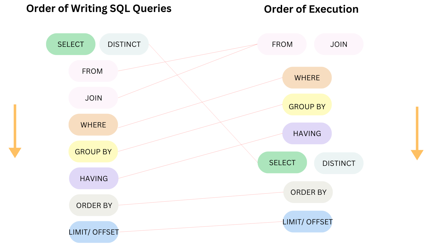
WHERE cannot see aggregates and HAVING can.
Wrong-query gallery #1
A colleague wants the industries that pay 40 dollars an hour or more on average, and writes:
%%sql
SELECT industry, AVG(hourly_wage) AS avg_wage
FROM survey
WHERE AVG(hourly_wage) >= 40
GROUP BY industry
RuntimeError: (sqlite3.OperationalError) misuse of aggregate: AVG()
[SQL: SELECT industry, AVG(hourly_wage) AS avg_wage
FROM survey
WHERE AVG(hourly_wage) >= 40
GROUP BY industry]
(Background on this error at: https://sqlalche.me/e/20/e3q8)This one does not fail silently: SQLite refuses to run it. Read the error message: misuse of aggregate. Why is an aggregate misused here?
Show / hide answer
Follow the evaluation order: WHERE runs before GROUP BY, at a point where the engine is looking at individual rows and no groups or averages exist yet, so an aggregate inside WHERE is meaningless and SQL rejects it. Filtering on an aggregate is exactly what HAVING is for. Enjoy this error, it is one of the few times SQL stops you instead of handing back a wrong number. The corrected syntax:
%%sql
SELECT industry, AVG(hourly_wage) AS avg_wage
FROM survey
GROUP BY industry
HAVING AVG(hourly_wage) >= 40| industry | avg_wage | |
|---|---|---|
| 0 | Construction | 40.484393 |
| 1 | Finance | 48.986667 |
| 2 | Public administration | 40.421190 |
| 3 | Technology | 48.957917 |
Four industries clear the bar.
Your turn. The team also wants education numbers. Using only the
surveytable: for each education level, return the number of respondents and their average hourly wage, best paid group first. Start the cell with%%sql. If it is right, it returns 4 rows, with graduate degrees on top at just over 50 dollars an hour.
# your query hereShow / hide answer
%%sql
SELECT education, COUNT(*) AS respondents, AVG(hourly_wage) AS avg_wage
FROM survey
GROUP BY education
ORDER BY avg_wage DESC| education | respondents | avg_wage | |
|---|---|---|---|
| 0 | Graduate degree | 121 | 50.133802 |
| 1 | Bachelor's degree | 269 | 42.645465 |
| 2 | College diploma | 319 | 36.004796 |
| 3 | High school | 291 | 32.879175 |
6. The wrong number we almost published
The briefing asks for regions, not provinces, so the real draft needs section 4’s join and section 5’s grouping working together.
Predict first. The lookup table maps five provinces into three regions. How many rows will the regional table have?
%%sql
SELECT p.region, COUNT(*) AS workers, AVG(s.hourly_wage) AS avg_wage
FROM survey AS s
JOIN provinces AS p ON s.province = p.province
GROUP BY p.region| region | workers | avg_wage | |
|---|---|---|---|
| 0 | Central Canada | 414 | 37.909396 |
| 1 | Prairies | 187 | 39.830267 |
| 2 | West Coast | 353 | 38.209887 |
Three regions, with sensible looking averages, a table you could paste straight into the report. Before we do, apply section 5’s habit and read the counts: 414 + 187 + 353 = 954. We surveyed 1,000 people. Where are the other 46?
Inner join dropped every respondent whose province has no row in provinces, and Saskatchewan has no row. Those people are findable, since the left join keeps them with NULL where a region should be. NULL is SQL’s marker for “no value here”, and it does not behave like a value. Watch what happens when we hunt for the missing rows with WHERE:
%%sql
SELECT s.respondent_id, s.province, p.region
FROM survey AS s
LEFT JOIN provinces AS p ON s.province = p.province
WHERE p.region = NULL| respondent_id | province | region |
|---|
Zero rows, even though we watched 46 of them appear in section 4. The query looks correct, SQL raised no error, and the rows just aren’t there. The reason for this is that: = NULL is never true, for anything, including NULL itself. NULL means “unknown”, and SQL’s logic is three-valued: a comparison can be true, false, or unknown, and any comparison against an unknown is itself unknown (think of this like undefined in math). WHERE keeps only the rows whose condition is true, so unknown is discarded just like false. Finding NULLs therefore has its own dedicated command, IS NULL (and its opposite, IS NOT NULL):
%%sql
SELECT COUNT(*) AS missing_region
FROM survey AS s
LEFT JOIN provinces AS p ON s.province = p.province
WHERE p.region IS NULL| missing_region | |
|---|---|
| 0 | 46 |
All 46, accounted for; excellent. Now the correct version of the regional draft. Rerun it with a left join, and GROUP BY does something helpful on its own: it collects all the NULLs into a group of their own:
%%sql
SELECT p.region, COUNT(*) AS workers, AVG(s.hourly_wage) AS avg_wage
FROM survey AS s
LEFT JOIN provinces AS p ON s.province = p.province
GROUP BY p.region| region | workers | avg_wage | |
|---|---|---|---|
| 0 | None | 46 | 42.616304 |
| 1 | Central Canada | 414 | 37.909396 |
| 2 | Prairies | 187 | 39.830267 |
| 3 | West Coast | 353 | 38.209887 |
The None row is Saskatchewan, and it has the highest average wage in the table. Our three-region draft omitted 46 individuals who were the highest paid group in the survey and skewed every comparison in the process. Nothing crashed, no error warned us, and the wrong table even looked cleaner than the right one.
NULL causes chaos outside databases too. In 2016 a security researcher registered the custom license plate NULL, and whenever officers left the plate field blank on a citation, the system matched it to him:

7. Comparing fairly: CASE
The briefing spec says full-time workers only, and the survey has hours, not a full-time indicator column. CASE is SQL’s if-else, and it builds new columns out of conditions. Use it whenever the category you want to analyze does not exist as a column yet: banding a continuous variable, collapsing detailed codes into coarse groups, or building a dummy variable. Statistics Canada draws the full-time line at 30 hours a week, so let us build it (we will call it work_status) and summarize both groups:
%%sql
SELECT CASE WHEN weekly_hours >= 30 THEN 'Full-time' ELSE 'Part-time' END AS work_status,
       COUNT(*) AS respondents,
       AVG(hourly_wage) AS avg_wage
FROM survey
GROUP BY work_status| work_status | respondents | avg_wage | |
|---|---|---|---|
| 0 | Full-time | 819 | 38.718083 |
| 1 | Part-time | 181 | 38.017017 |
819 full-timers, 181 part-timers, similar hourly wages. Notice the composition: CASE invents a column that exists nowhere in the table, and GROUP BY groups on it. A CASE can also hold many WHEN branches, checked top to bottom with the first match winning, which is how you band a numeric column into exclusive groups.
8. The final deliverable
We are ready! The end product we need is: wages by region, full-time workers only, with worker counts and union shares, and we will report only regions with at least 50 such workers. Two small things appear inside it. ROUND(value, 2) rounds a number to the given count of decimal places, two here, so the summary columns come back readable instead of trailing twelve decimals. And for the union share we will do a simple trick: union_member holds 0 or 1, and the average of a 0/1 column is a share, so AVG(s.union_member) is exactly the union share we need.
%%sql
SELECT p.region,
       COUNT(*) AS workers,
       ROUND(AVG(s.hourly_wage), 2) AS avg_wage,
       ROUND(AVG(s.union_member), 2) AS union_share
FROM survey AS s
LEFT JOIN provinces AS p ON s.province = p.province
WHERE s.weekly_hours >= 30
GROUP BY p.region
HAVING COUNT(*) >= 50
ORDER BY avg_wage DESC| region | workers | avg_wage | union_share | |
|---|---|---|---|---|
| 0 | Prairies | 157 | 39.83 | 0.25 |
| 1 | Central Canada | 343 | 38.34 | 0.30 |
| 2 | West Coast | 283 | 38.16 | 0.26 |
Read it in evaluation order, the same list from section 5: the join builds person-region rows, WHERE keeps the 819 full-timers, GROUP BY folds them into regions, HAVING keeps regions with 50 or more, SELECT computes and rounds the summaries, and ORDER BY sorts the surviving entries.
Think Deeper.
AVG(union_member)works because the mean of a dummy variable is a proportion. You have used this fact all through your econometrics education: it is why a regression of a 0/1 outcome on a constant returns the sample share. The trick carries over to any yes/no column you encounter.
One thing to consider: Saskatchewan’s full-timers, 36 of them, formed a NULL-region group, and the 50-worker floor in HAVING dropped it. That is the same group that we lost in section 6, but with one difference: this time we know, we chose the threshold, and we state this clearly in the meeting and final report. Dropping data can be okay, and sometimes it’s the correct choice outright. Dropping data without knowing is how wrong numbers get published and is always bad.
9. The question we cannot answer yet
The report is out, and a co-worker immediately asks the natural follow-up: do certified workers earn more? We have a certifications table; it feels like one join away.
It depends on a definition. The grain of a table is what one row stands for. In survey, a row is a person; in the certification join from section 4.3, a row is a person-certification pair. Aggregates count rows, so they answer questions at the grain of the table they are given, whether or not that is the question you asked.
Wrong-query gallery #2
How many respondents hold at least one certification? A colleague joins and counts:
%%sql
SELECT COUNT(*) AS certified_respondents
FROM survey AS s
JOIN certifications AS c ON s.respondent_id = c.respondent_id| certified_respondents | |
|---|---|
| 0 | 684 |
684 certified respondents. What is wrong, and what is the real number?
Show / hide answer
684 is the number of certifications, because the join has one row per person-certification pair and respondent 8 is being counted once per certificate. The question asks about people, and COUNT(DISTINCT s.respondent_id) counts each person once. Whenever a query involves a join, decide what one row means before you aggregate. The corrected syntax:
%%sql
SELECT COUNT(DISTINCT s.respondent_id) AS certified_respondents
FROM survey AS s
JOIN certifications AS c ON s.respondent_id = c.respondent_id| certified_respondents | |
|---|---|
| 0 | 452 |
The real number is 452.
Counting people was rescued by COUNT(DISTINCT ...). The average wage is where this breaks:
%%sql
SELECT AVG(s.hourly_wage) AS avg_wage_certified
FROM survey AS s
JOIN certifications AS c ON s.respondent_id = c.respondent_id| avg_wage_certified | |
|---|---|
| 0 | 39.894459 |
39.89 dollars an hour, and we know before publication that it is computed at the wrong grain: every multi-certificate respondent’s wage is counted once per certificate, so the heavily certified pull the average toward themselves. What we want is the average over one row per certified person. With this notebook’s tools, a single SELECT, we are stuck. You would need to first collapse the join down to one row per person, and then average the result, which means running a query on the output of another query. A query inside a query.
That is exactly where Notebook 3 begins.
10. Conclusion
The briefing shipped, and it was correct! Getting one table right took joins, aggregates, group filters, a manufactured column, and three close calls: a hunt for missing rows that came back empty because = NULL is never true, an inner join that deleted the best-paid group in the data, and a count taken at the wrong grain. They were queries that ran without throwing an error.
Thanks for sticking with me; SQL is the language of modern data and databases. It is a useful skill and the language itself is very human-readable with limited obfuscations and weird issues (most of which we discussed above). The coming notebooks will be more fun with more interesting real life examples. This notebook was much more computer science and code syntax, but it is worth it! With a little more practice you can write SQL as a skill on your resume and a whole bunch of jobs after graduation open up for you.
You can now answer these interview questions
- What is the difference between an inner join and a left join, and how can a join change the number of rows?
- Why can
COUNT(column)be smaller thanCOUNT(*)? - When do you filter with
WHEREand when withHAVING? - Why does
WHERE x = NULLreturn nothing, and what do you write instead?
Show / hide model answers
- An inner join keeps only rows that find a match; a left join keeps every left-table row and fills unmatched columns with NULL. Row counts shrink when rows fail to match, and grow when a row matches several partners, one output row per matching pair.
COUNT(*)counts rows;COUNT(column)counts only non-NULL values in that column, so every NULL widens the gap.WHEREfilters individual rows before grouping and cannot see aggregates;HAVINGfilters whole groups afterGROUP BYand can.- Comparisons with NULL evaluate to unknown rather than true, so the filter keeps nothing; write
x IS NULL(orx IS NOT NULL).
Appendix: where to practice
Everything in this notebook is interview material, and the way to make it permanent is repetitions on someone else’s data and questions. Three free sites are the standard tools:
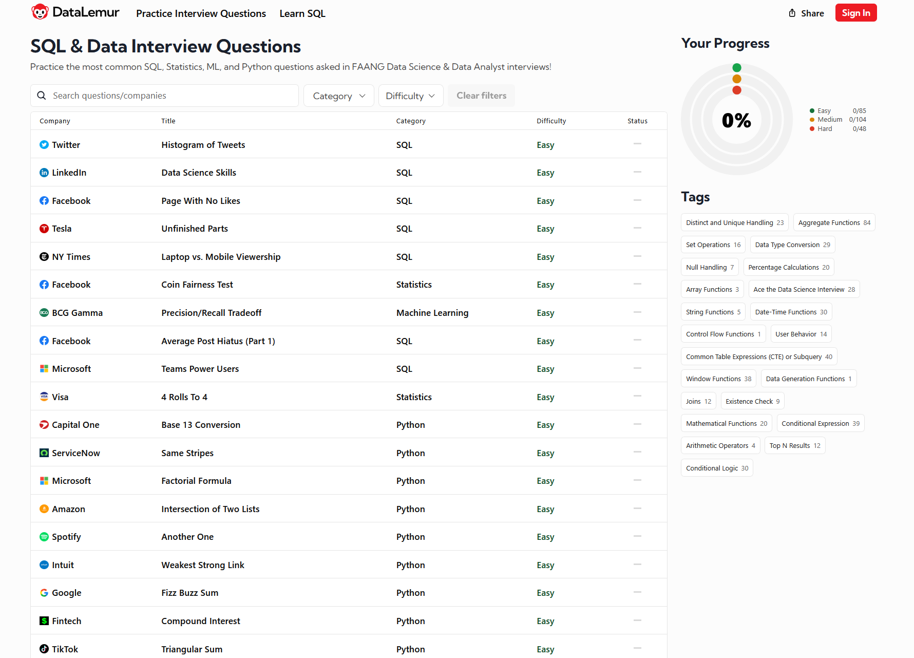
- DataLemur: SQL questions taken from real company interviews, with a generous free tier.
- StrataScratch: interview questions you can solve in SQL or Python
pandas. - LeetCode SQL 50: the classic curated list; its easy tier maps almost exactly onto this notebook.
You are ready for the easy tier of all three right now: it is SELECT, WHERE, joins, and GROUP BY, which is what we just learned.
Connections
- Back to Notebook 1: there we built the database and asked one-table questions; here the database grew to three tables.
- Forward to Notebook 3: the certified-wage question needs a query that runs on the output of another query. Subqueries, CTEs, and views, window functions, changing data with INSERT and UPDATE, and how to run SQL from Python safely, including what a SQL injection is.
References
- Government of Canada. Current and forthcoming general minimum wage rates in Canada. https://minwage-salairemin.service.canada.ca/en/general.html The source of the minimum wages in
provinces.csv(rates in force April 2025). - Malan, D. (2024). CS50’s Introduction to Databases with SQL. Harvard University. https://cs50.harvard.edu/sql/ (Lecture 1, Relating, covers joins.)
- ThoughtSpot (formerly Mode). SQL tutorial. https://www.thoughtspot.com/sql-tutorial A free reference that extends everything here.
- SQLite. The SELECT statement. https://www.sqlite.org/lang_select.html
- SQLite. NULL handling in SQLite. https://www.sqlite.org/nulls.html Three-valued logic, from the engine’s own documentation.
- Statistics Canada. Average weekly earnings, average hourly wage rate and average usual weekly hours by union status, annual. Table 14-10-0134-01. https://www150.statcan.gc.ca/t1/tbl1/en/tv.action?pid=1410013401 The real-world version of this notebook’s deliverable, shown in section 1.
- Statistics Canada. (2025). Canada’s population estimates, first quarter 2025. The Daily, June 18, 2025. https://www150.statcan.gc.ca/n1/daily-quotidien/250618/dq250618a-eng.htm The source of the populations in
provinces.csv.