# # Core packages
# !pip install \
#     datasets==3.6.0 \
#     transformers \
#     pandas \
#     numpy \
#     statsmodels \
#     holidays \
#     plotly \
#     ipywidgets \
#     scikit-learn \
#     matplotlib \
#     seaborn \
#     torch \
#     yfinance
# !pip3 install torch torchvision --index-url https://download.pytorch.org/whl/cpu --quietHow Do Large Language Models Predict?
ECON 227
Python
large language models
prediction
This notebook explores how large language models (LLMs) work by linking their probability-based predictions to real-world applications. We start with the basics of next-word prediction, then extend the idea to forecasting stock prices using news sentiment.
Learning Outcomes
By the end of this notebook, students will be able to:
- Understand next-word prediction as a conditional probability distribution over a model’s vocabulary
- Explain how temperature controls the sharpness of that distribution and shapes a model’s outputs
- Apply a pretrained sentiment classifier to financial text and evaluate it with a confusion matrix
- Interpret confidence scores and their relationship to accuracy
- Use sentiment features in a simple linear regression to predict stock returns
Prerequisites
Before you start, make sure you have the required libraries installed, if not, uncomment the lines below (i.e. remove the #) and run the cell to install them:
Important: Run this cell to load the libraries we need for running this notebook.
# load libraries we need to run this notebook
import os
import warnings
import numpy as np
import pandas as pd
import matplotlib.pyplot as plt
import seaborn as sns
import yfinance as yf
from transformers import pipeline, AutoTokenizer, AutoModelForCausalLM
import torch
import torch.nn.functional as F
from sklearn.metrics import confusion_matrix, ConfusionMatrixDisplay, classification_report
1 Introduction: The Mathematics of LLM Predictions
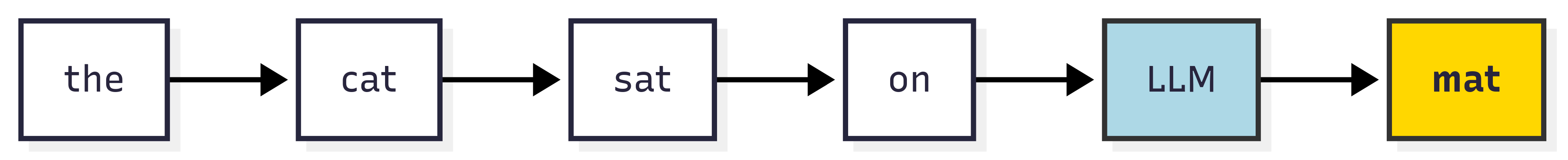
Large language models like ChatGPT do something that seems very simple: Next word prediction.
What does that mean? It means that given a sequence of words, the model predicts the next word in the sequence. For example, if the input is “The cat sat on the…”, the model might predict “mat” as the next word.
This is an example of predicting just one word. While these models predict only one word at a time, they can do this for very long sequences of words.
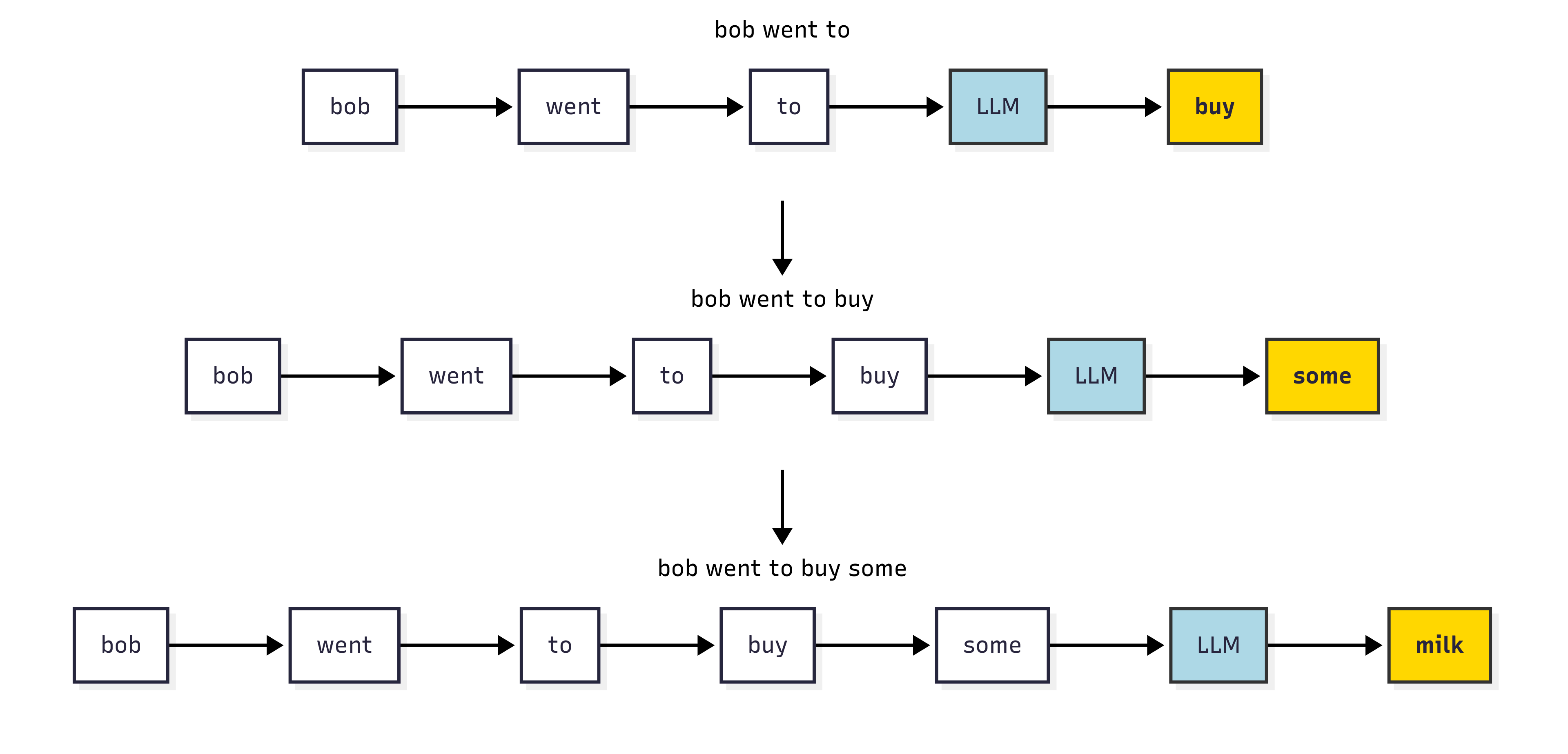
For example, consider completing: “Bob went to…”
Suppose we want to output a total of \(T\) words to form a sentence. We can represent the words (\(w\)) in the sentence as \(w_1, w_2, \ldots, w_t, \ldots, w_{T-1}, w_T\) where subscript \(t\) means the word (\(w_t\)) is at the position \(t\).
The model tries to learn the probability distribution of the next word given the previous words. It seeks to create a list of numbers between 0 and 1, one for each possible next word, that together add up to 1. These numbers are the probability of choosing that word as the next word in the sentence.
Given the previous words \(w_1, w_2, \ldots, w_{t-1}\), the probability of predicting the next word \(w_{t}\) is called conditional probability: it measures for all words in the vocabulary “the probability of this word being next, based on what was already said”.
Mathematically, this is just the definition of a conditional probability:
\[ P(w_t \mid w_1, w_2, \ldots, w_{t-1}) = \frac{P(w_1, w_2, \ldots, w_{t-1}, w_t)}{P(w_1, w_2, \ldots, w_{t-1})} \]
LLMs estimate this probability by learning from training datasets. When they make predictions, they will select the word at position \(t\) as the word with the highest probability to be the next word. Some models also choose likely words at random, which can lead to more creative outputs.
Let’s see how this works in practice. The code below sets up a simple example of assigning the next word in the sentence “Bob went to the…” at each step, and shows how the probability distribution changes as we add more words to the sentence. We use a very small vocabulary to make it easier to visualize.
Note: the probabilities below are hand-picked to illustrate the idea; in a real model, these would be learned from training data.
warnings.filterwarnings("ignore")

# Example vocabulary
vocab = ['buy', 'some', 'milk', 'along', 'the', 'way']

# Probabilities at each step (example)
probs_step1 = [0.8, 0.05, 0.05, 0.03, 0.04, 0.03]  # 'buy' high
probs_step2 = [0.05, 0.7, 0.1, 0.05, 0.05, 0.05]   # 'some' high
probs_step3 = [0.05, 0.05, 0.75, 0.05, 0.05, 0.05] # 'milk' high

prob_distributions = [probs_step1, probs_step2, probs_step3]
step_labels = ['Step 1: Predict "buy"', 'Step 2: Predict "some"', 'Step 3: Predict "milk"']

fig, axes = plt.subplots(3, 1, figsize=(8, 8), sharey=True)

for i, ax in enumerate(axes):
    sns.barplot(x=vocab, y=prob_distributions[i], palette='muted', ax=ax)
    ax.set_title(step_labels[i])
    ax.set_ylim(0, 1)
    ax.set_ylabel('Probability' if i == 0 else '')
    ax.set_xlabel('Vocabulary')
    # Highlight the max prob bar in gold
    max_idx = prob_distributions[i].index(max(prob_distributions[i]))
    ax.bar(max_idx, prob_distributions[i][max_idx], color='gold')

    for patch, token, prob in zip(ax.patches, vocab, prob_distributions[i]):
        height = patch.get_height()
        ax.annotate(
            f"{prob:.2f}",
            xy=(patch.get_x() + patch.get_width() / 2, height),
            xytext=(0, 3),
            textcoords="offset points",
            ha='center', va='bottom',
            fontsize=9
        )

plt.tight_layout()
plt.show()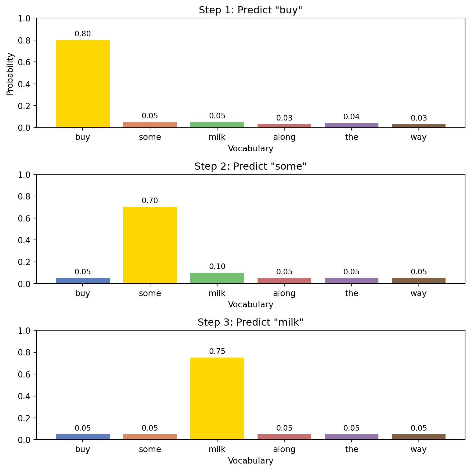
We can also use a “real” example with a pre-trained language model, which has a much larger vocabulary and can handle more complex sentences. The code below uses a model from Hugging Face, which is a popular platform for sharing machine learning models.
# Load a pre-trained model and tokenizer from Hugging Face
Next_word_prediction = "distilbert/distilgpt2"
tokenizer = AutoTokenizer.from_pretrained(Next_word_prediction)
model = AutoModelForCausalLM.from_pretrained(Next_word_prediction)
model.eval()

device = torch.device("cuda" if torch.cuda.is_available() else "cpu")
model.to(device)
print("Loaded:", Next_word_prediction, "on", device)
Loaded: distilbert/distilgpt2 on cpuLet’s use the model to predict the next word in a sentence.
Try changing the sentence below to see how the predicted next word changes.
predict_next_word("The cat sat on the")Sentence: The cat sat on the
Prediction (top-1): ' floor' | prob = 0.065
' floor' 0.065
' bed' 0.064
' couch' 0.055
' table' 0.052
' back' 0.0512 Sampling and Temperature
The example above (“Bob went to…”) shows the process of generating a short sentence. At each step, the model calculates the conditional probability of the next word and then selects the word with the highest probability to insert into the sentence. The final output we obtain, in our hand-picked example is: “buy some milk”.
To get more creative responses you can change the way you pick the next word: pick a “likely” word but not necessarily the most probable one. Simply put, this involves making the conditional distribution sharper or flatter. If you make the distribution sharper, you are more likely to pick the word with the highest probability. If you make it flatter, you are more likely to pick a word that is not the most probable one.
This is called temperature. A higher temperature makes the distribution flatter, while a lower temperature makes it sharper. You would want to use a temperature of more than one \((1.2-1.5)\) for creative responses, and a temperature of less than one \((0.1 - 0.5)\) for more focused responses. For a balanced response, you can use a temperature of \(0.7-1\). There are other options that can also be adjusted, but temperature is the most common.
Let’s see another example, using a small vocabulary and a simple sentence, to see how the probability distribution changes with different temperatures.
warnings.filterwarnings("ignore")

np.random.seed(42)

# Example vocabulary
vocab = [
    'apple', 'banana', 'cherry', 'date', 'elderberry',
    'fig', 'grape', 'honeydew', 'kiwi', 'lemon',
    'mango', 'nectarine', 'orange', 'papaya', 'quince',
    'raspberry', 'strawberry', 'tangerine', 'ugli', 'watermelon'
]

# Normalize to sum to 1
vocab_size = len(vocab)
base_probs = np.random.rand(vocab_size)
base_probs /= base_probs.sum()

def apply_temperature(probs, temp):
    logits = np.log(probs + 1e-20)
    scaled_logits = logits / temp
    exp_logits = np.exp(scaled_logits)
    return exp_logits / exp_logits.sum()

temperatures = [0.5, 1.0, 1.5]
distributions = [apply_temperature(base_probs, t) for t in temperatures]

fig, axes = plt.subplots(3, 1, figsize=(8, 8), sharey=True)
for i, (ax, dist, temp) in enumerate(zip(axes, distributions, temperatures)):
    sns.barplot(x=vocab, y=dist, palette='muted', ax=ax)
    ax.set_title(f'Temperature = {temp}')
    ax.set_ylim(0, 0.25)
    ax.set_ylabel('Probability' if i == 0 else '')
    ax.set_xlabel('Vocabulary')
    ax.tick_params(axis='x', rotation=90)

    # Highlight the max-prob bar in gold
    max_idx = dist.argmax()
    ax.patches[max_idx].set_color('gold')

    # Annotate each bar with its probability
    for patch, prob in zip(ax.patches, dist):
        height = patch.get_height()
        ax.annotate(
            f"{prob:.2f}",
            xy=(patch.get_x() + patch.get_width() / 2, height),
            xytext=(0, 3),            # 3 points vertical offset
            textcoords="offset points",
            ha='center', va='bottom',
            fontsize=9
        )

plt.tight_layout()
plt.show()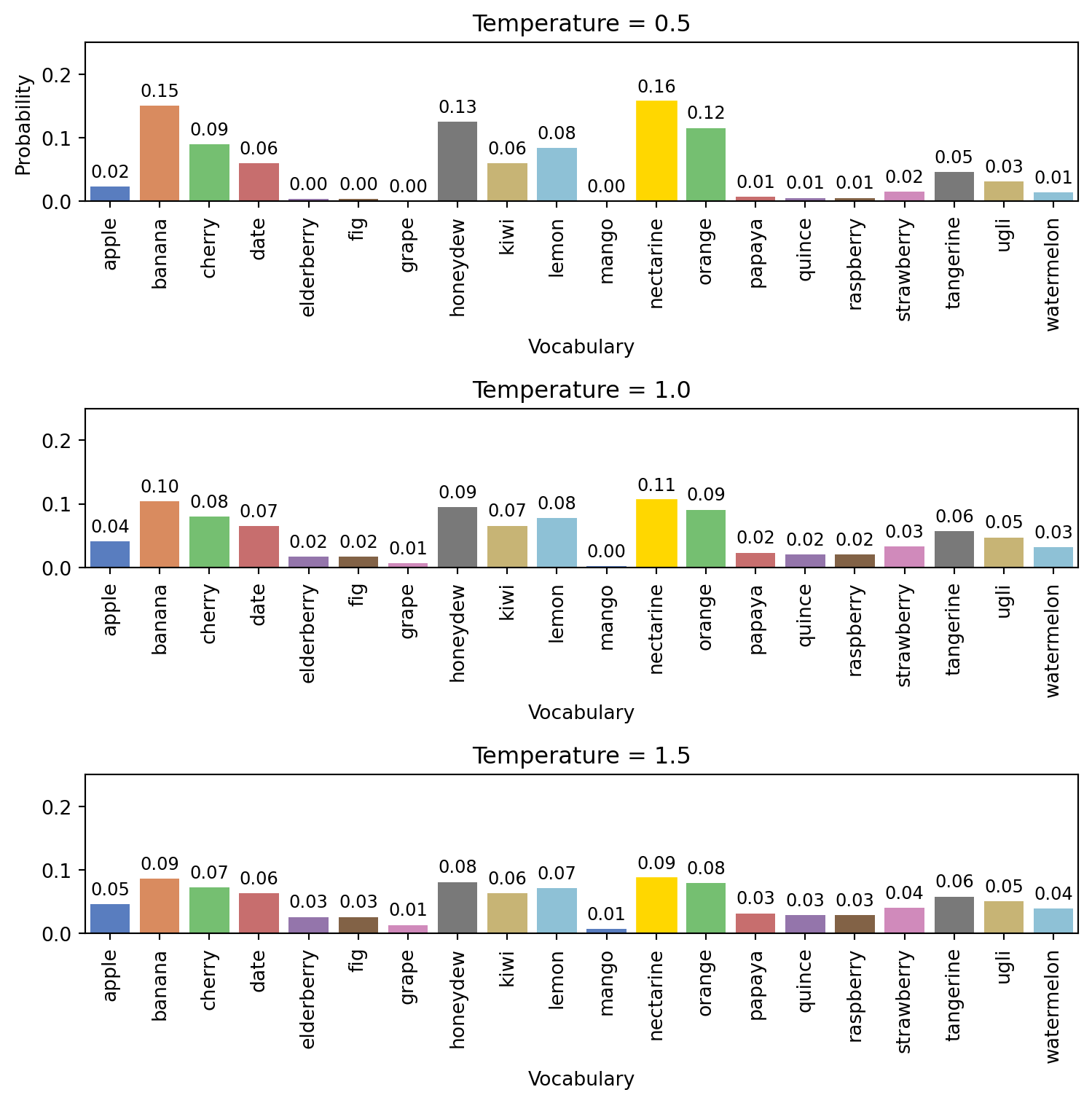
In the example above, we see how the probability distribution changes with different temperatures. A high temperature (1.5) results in a flatter distribution, meaning the model is more likely to sample from less probable tokens, while a low temperature (0.5) results in a sharper distribution, favoring the most probable tokens.
Again, we can see this with our pre-trained model from Hugging Face.
Now, let’s apply the same idea to our own sentence using a real language model.
Try changing the sentence or the temperature below to see how the distribution changes.
Predict first
Before you bump the temperature to 1.5: does the gold bar get taller or shorter?
Answer
Shorter. Higher temperature flattens the distribution, it pulls weight off the top token onto the rest.
# change the value after "temperature = " to see how the distribution changes with different temperatures
plot_next_token_distribution("The cat sat on the", temperature = 1.0)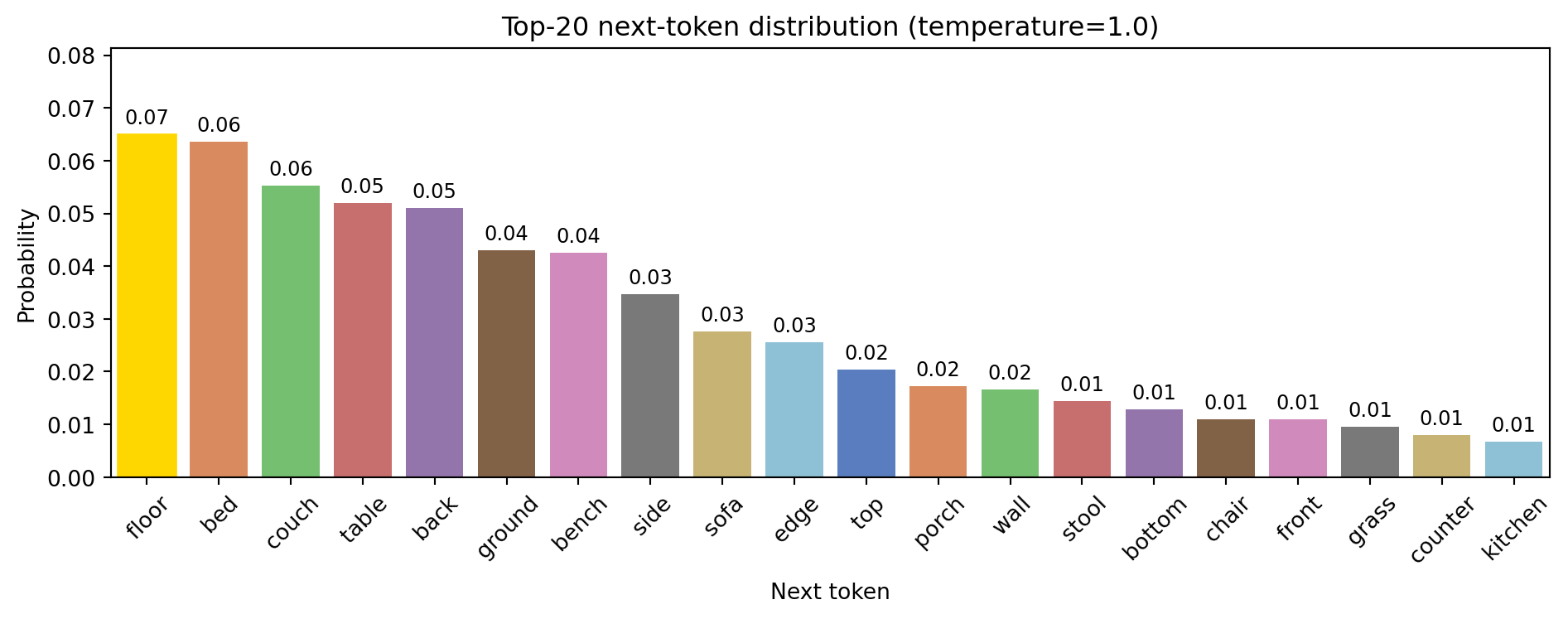
If you are interested in understanding the inner workings of these models, take a look at the interactive visualization at The Illustrated Transformer. It provides an excellent, hands-on way to explore the core ideas behind modern language models.
While our examples here use words and sentences, the same idea applies to any sequential data such as stock prices, weather, or moves in a game like chess. The model looks at what happened before and tries to guess what comes next.
So, just like a model guesses the next word in a sentence, it can also guess the next day’s temperature or the next movement in a stock price, based on the pattern it sees in the earlier numbers.
Here is a simple example of how a model might predict stock prices over time, showing the actual data, the predicted values, and the uncertainty around those predictions.
n = 10
m = 9

# Generate actual data: random walk + small trend
actual_data = np.cumsum(np.random.normal(0, 1, n)) + 50

# Predictor approximates entire data closely with small noise everywhere
predicted = actual_data + np.random.normal(0, 0.2, n)

# Posterior uncertainty: low and roughly constant over entire period
posterior_std = np.full(n, 0.3)

upper = predicted + posterior_std
lower = predicted - posterior_std

plt.figure(figsize=(6,6))
plt.plot(range(n), actual_data, label="Actual Data", color='blue')
plt.plot(range(n), predicted, label="Predicted", color='orange')
plt.axvline(x=m-1, color='black', linestyle='--', label="Observed / Future Split")

plt.xlabel("Time")
plt.ylabel("Value")
plt.title("Stock price over time.")
plt.legend()
plt.show()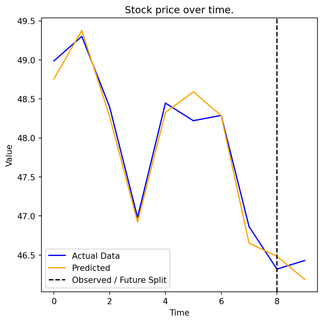
Typically, when building a model to predict something like stock prices, you would use more information than just the past prices. For example, you might include things like public sentiment (how people feel about the stock), news headlines, or other features that could influence the price. Predicting words also can use more information than just the previous words: it can use the overall topic, the style of writing, or even the intended audience.
3 Classifying Headline Sentiment with LLM
Earlier, we explored how large language models (LLMs) predict the next word by learning the probability distribution of possible outcomes based on context.
Now, we apply a similar idea to entire sentences: in this case, financial news headlines. Instead of predicting the next word, we want to predict whether a sentence is positive, negative, or neutral. Specifically, we want the model to assign a probability to each sentiment category: POSITIVE, NEGATIVE, or NEUTRAL.
So, instead of predicting the next word given the previous words, we are now predicting the sentiment given the words in the headline. Instead of:
\[ P(w_t \mid w_1, w_2, \ldots, w_{t-1}) \]
We now predict:
\[ P( \text{Sentiment} \mid \text{Headline}) \]
Intuitively, we are asking the model:
Given the words in this sentence, what is the most likely emotion behind it?
How it works:
- Our model reads the headline.
- Based on the words and their context, it calculates the probability of the headline being positive, negative, or neutral.
- It then assigns the headline to the category with the highest probability, and also gives us a confidence score (the probability of that category).
To do this, we will use some models that have already been trained to do this task well. Specifically, we will use a model called RoBERTa (short for Robustly Optimized BERT Pretraining Approach). RoBERTa is a pretrained language model that learns a word’s meaning by looking at the words before and after it, so it understands context and tone well. It is also specifically trained on tweets and social media text, so it tends to be well-suited to handling short, non-technical texts like news headlines.
Our plan is to build on our earlier discussion of LLMs predicting probability distributions, but here, the prediction is over sentiment classes rather than words. This process converts unstructured text into structured sentiment labels that we can analyze quantitatively, making it a useful complement to other kinds of data in economic or statistical analysis.
We now apply our pre-trained model to each headline. It will return either:
POSITIVE: news that sounds good (e.g., “profits surge”)NEGATIVE: news that sounds bad (e.g., “lawsuit filed”)NEUTRAL: news that is neither clearly negative nor positive.
Can you think of a positive and negative news headline?
warnings.filterwarnings("ignore")
# Here we are just specifying the classifier (AI model) that decides on a sentiment

classifier = pipeline("sentiment-analysis", model="cardiffnlp/twitter-roberta-base-sentiment-latest", device=-1)

# define a function to classify sentiment of each text
def classify_sentiment(text):
    return classifier(text)[0]["label"].upper()

# we'll also define a helper that returns the confidence score of the model.
def classify_with_score(text):
    result = classifier(str(text), truncation=True, max_length=512)[0]
    return result["label"].upper(), result["score"]
WARNING:tensorflow:From D:\Users\alexr\anaconda3\Lib\site-packages\tf_keras\src\losses.py:2976: The name tf.losses.sparse_softmax_cross_entropy is deprecated. Please use tf.compat.v1.losses.sparse_softmax_cross_entropy instead.
Some weights of the model checkpoint at cardiffnlp/twitter-roberta-base-sentiment-latest were not used when initializing RobertaForSequenceClassification: ['roberta.pooler.dense.bias', 'roberta.pooler.dense.weight']
- This IS expected if you are initializing RobertaForSequenceClassification from the checkpoint of a model trained on another task or with another architecture (e.g. initializing a BertForSequenceClassification model from a BertForPreTraining model).
- This IS NOT expected if you are initializing RobertaForSequenceClassification from the checkpoint of a model that you expect to be exactly identical (initializing a BertForSequenceClassification model from a BertForSequenceClassification model).
Device set to use cpu
Before seeing what the model says, let’s test our own intuition. Given the headlines below, would you say they are positive, negative, or neutral?
headlines = [
    "Operating profit rose to EUR 17.1 mn from EUR 14.8 mn in the corresponding period of 2007.",
    "The company was ordered to pay damages worth 8.8 million euros.",
    "Sales for the third quarter were flat compared to the same period last year.",
    "The rights issue was subscribed to 102 percent.",
    "The company faces a wave of new lawsuits following the product recall.",
    "Quarterly revenue in line with market expectations.",
    "SVB Financial Group, the former parent company of Silicon Valley Bank, filed for Chapter 11 bankruptcy in March 2023 following the bank's collapse and FDIC receivership"
]
Okay, now what does RoBERTa say about these headlines? Let’s see:
print("Roberta's Sentiment Analysis\n" + "=" * 60)
for headline in headlines:
    label, score = classify_with_score(headline)
    print(f"\nHeadline : {headline}")
    print(f"Predicted: {label}  (confidence: {score:.2f})")
Roberta's Sentiment Analysis
============================================================
Headline : Operating profit rose to EUR 17.1 mn from EUR 14.8 mn in the corresponding period of 2007.
Predicted: NEUTRAL (confidence: 0.68)
Headline : The company was ordered to pay damages worth 8.8 million euros.
Predicted: NEGATIVE (confidence: 0.62)
Headline : Sales for the third quarter were flat compared to the same period last year.
Predicted: NEUTRAL (confidence: 0.73)
Headline : The rights issue was subscribed to 102 percent.
Predicted: NEUTRAL (confidence: 0.86)
Headline : The company faces a wave of new lawsuits following the product recall.
Predicted: NEGATIVE (confidence: 0.65)
Headline : Quarterly revenue in line with market expectations.
Predicted: NEUTRAL (confidence: 0.71)
Headline : SVB Financial Group, the former parent company of Silicon Valley Bank, filed for Chapter 11 bankruptcy in March 2023 following the bank's collapse and FDIC receivership
Predicted: NEGATIVE (confidence: 0.62)Do you agree with the model’s predictions? Why or why not? If it seems to have got it wrong, can you think of why? What words or phrases might have confused the model?
4 Applying Sentiment Classification to Real News
Thus far, we’ve applied our sentiment classifier to a handful of example sentences. But it’s likely your own opinion on at least a few of these sentences differed from the model’s opinion. Who is right? In particular, how reliable is the model on actual financial texts?
To answer that, we’ll use the financial phrasebank, a benchmark dataset frequently used in natural language research. The dataset contains 3,435 financial news sentences that have been gathered from financial news archives. Each sentence has been labelled as positive, negative or neutral by a panel of domain experts in finance. We use the version where at least 75% of the annotators agreed on the label to ensure a somewhat objective “true” label.
Here are the details of the dataset:
phrasebank_df = pd.read_csv("datasets/phrasebank_full.csv")

print(f"size of dataset: {len(phrasebank_df)} sentences")
print(f"\nlabel distribution:")
print(phrasebank_df["true_label"].value_counts())
phrasebank_df[["sentence", "true_label"]].head()
size of dataset: 3453 sentences
label distribution:
true_label
NEUTRAL 2146
POSITIVE 887
NEGATIVE 420
Name: count, dtype: int64| sentence | true_label | |
|---|---|---|
| 0 | According to Gran , the company has no plans t... | NEUTRAL |
| 1 | With the new production plant the company woul... | POSITIVE |
| 2 | For the last quarter of 2010 , Componenta 's n... | POSITIVE |
| 3 | In the third quarter of 2010 , net sales incre... | POSITIVE |
| 4 | Operating profit rose to EUR 13.1 mn from EUR ... | POSITIVE |
Let’s take a look at a few examples within this dataset.
for _, row in phrasebank_df.sample(5, random_state=42).iterrows():
    print(f"Label: {row['true_label']}  Sentence: {row['sentence']}")
Label: POSITIVE Sentence: Turnover surged to EUR61 .8 m from EUR47 .6 m due to increasing service demand , especially in the third quarter , and the overall growth of its business .
Label: NEUTRAL Sentence: In June it sold a 30 percent stake to Nordstjernan , and the investment group has now taken up the option to acquire EQT 's remaining shares .
Label: NEUTRAL Sentence: Aspo 's Group structure and business operations are continually developed without any predefined schedules .
Label: NEUTRAL Sentence: The device can also be used for theft protection and positioning of vehicles , boats and other assets .
Label: POSITIVE Sentence: Of the price , Kesko 's share is 10 mln euro $ 15.5 mln and it will recognize a gain of 4.0 mln euro $ 6.2 mln on the disposal which will be included in the result for the second quarter of 2008 .Running the classifier
We’ll now apply the RoBERTa model to each sentence. This will give us both a predicted label and a confidence score (the model’s probability for its chosen label). We’ll classify a balanced sample of 150 sentences per class, but if you want to run this on the full dataset just remove .apply(sample_group).
Note: running this code may take some time. If you’re running this code a second time, feel free to comment out the first 5 lines
sample_df = pd.concat(
        [grp.sample(min(150, len(grp)), random_state=42)
        for _, grp in phrasebank_df.groupby("true_label")],
        ignore_index=True) #don't reassign sample_df to phrasebank_df if you don't want a sample, or change 150 to some other number for a larger (or smaller) sample.

results = [classify_with_score(x) for x in sample_df["sentence"]]
sample_df["pred_label"] = [r[0] for r in results]
sample_df["confidence"] = [r[1] for r in results]
sample_df.to_csv("datasets/phrasebank_predictions.csv", index=False)
phrasebank_df = sample_df

phrasebank_df[["sentence", "true_label", "pred_label", "confidence"]].head()| sentence | true_label | pred_label | confidence | |
|---|---|---|---|---|
| 0 | The situation of coated magazine printing pape... | NEGATIVE | NEGATIVE | 0.801002 |
| 1 | Alma Media 's operating profit amounted to EUR... | NEGATIVE | NEUTRAL | 0.793037 |
| 2 | Reported operating margin was a negative 5.9 % . | NEGATIVE | NEGATIVE | 0.623730 |
| 3 | Sales by Seppala diminished by 6 per cent . | NEGATIVE | NEGATIVE | 0.655835 |
| 4 | HELSINKI Thomson Financial - Shares in Cargote... | NEGATIVE | NEGATIVE | 0.725927 |
How did the model do? Do you think it did well? Which sentences did it get right, and which did it get wrong? Can you see any patterns in the sentences that it struggled with?
One problem with this kind of evaluation is that it is hard to get a sense of the overall performance of the model just by looking at a few examples. To get a better sense of how well the model is doing, let’s see a common evaluation metric that summarizes the model’s performance across all sentences.
Confusion matrices
A confusion matrix gives us an overview of how often the model agrees with the expert labels. It also tells us when it makes a mistake, what label it predicted instead of the correct one. In the matrix, each row represents the true label, and each column is what the model predicted. A perfect model would have a diagonal matrix with 1s on the diagonal and 0s everywhere else.
cm = confusion_matrix(phrasebank_df["true_label"], phrasebank_df["pred_label"], labels=["POSITIVE", "NEUTRAL", "NEGATIVE"])

fig, ax = plt.subplots(figsize=(7, 5))
disp = ConfusionMatrixDisplay(confusion_matrix=cm, display_labels=["POSITIVE", "NEUTRAL", "NEGATIVE"])
disp.plot(ax=ax, colorbar=False, cmap="Greens")
ax.set_title("RoBERTa vs. the experts, financial phrasebank dataset")
plt.tight_layout()
plt.show()

print(classification_report(phrasebank_df["true_label"], phrasebank_df["pred_label"], labels=["POSITIVE", "NEUTRAL", "NEGATIVE"]))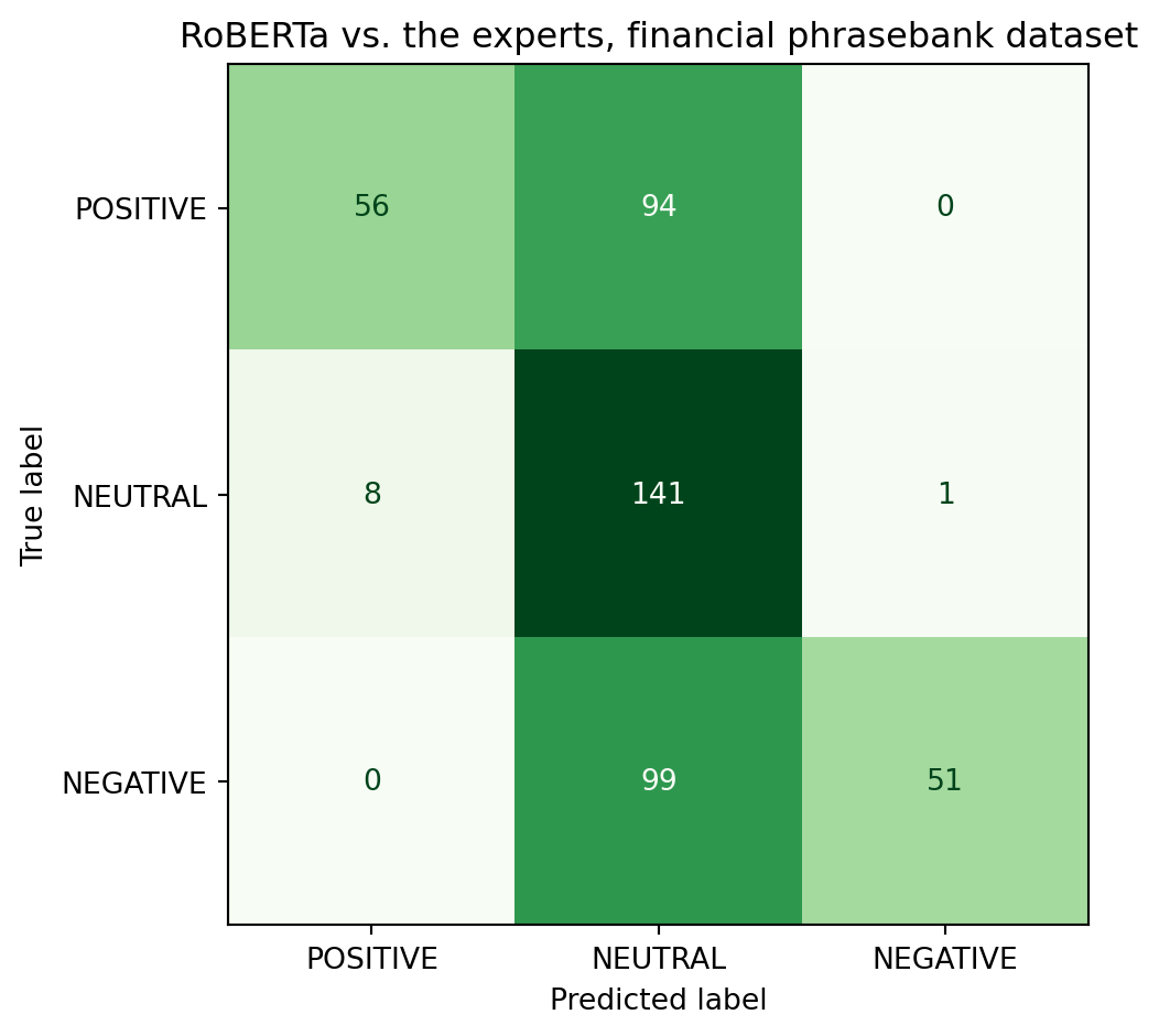
              precision    recall  f1-score   support

    POSITIVE       0.88      0.37      0.52       150
     NEUTRAL       0.42      0.94      0.58       150
    NEGATIVE       0.98      0.34      0.50       150

    accuracy                           0.55       450
   macro avg       0.76      0.55      0.54       450
weighted avg       0.76      0.55      0.54       450
Which class does the model struggle with the most? Why might that be?
Does confidence necessarily predict accuracy?
Recall that LLMs produce a probability distribution over all possible outcomes. The confidence score is the probability that the model assigns to its top prediction. In this section, let’s test whether that probability carries any real information. In other words, is the model more confident when it is correct or when it’s wrong?
Keep the results of this section in mind when a LLM tells you that it’s certain about something you ask it
(^_~)
phrasebank_df["correct"] = phrasebank_df["pred_label"] == phrasebank_df["true_label"] #new boolean column for when model is correct vs when it isnt


fig, ax = plt.subplots(figsize=(9,5))

ax.hist(phrasebank_df[phrasebank_df['correct']]['confidence'], bins=100, alpha=0.7, color="green",density=True, label="Model got correct prediction")

ax.hist(phrasebank_df[~phrasebank_df['correct']]['confidence'], bins=100, alpha=0.7, color="tomato",density=True, label="Model got incorrect prediction")

ax.set_xlabel("Model confidence score")
ax.set_ylabel("Density")
ax.set_title("Confidence Score Distribution")
ax.legend()
plt.tight_layout()
plt.show()

print(f"Mean confidence — correct:   {phrasebank_df[phrasebank_df['correct']]['confidence'].mean()}")
print(f"Mean confidence — incorrect: {phrasebank_df[~phrasebank_df['correct']]['confidence'].mean()}")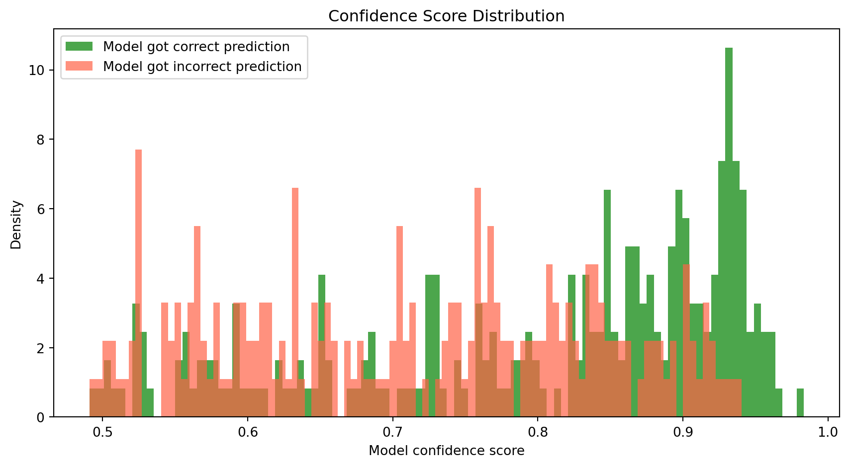
Mean confidence — correct:   0.8021508035880904
Mean confidence — incorrect: 0.7149594842207314
We see that a model’s probability score isn’t cosmetic: when it’s wrong, it’s more likely to be less sure, but not always so!
Predicting stock returns with sentiment data
In the last section, we validated our classifier on expert-labelled data. So far it’s okay, but not ideal. We saw that it can make some mistakes. Now, let’s apply it to something noisier and more informal: financial social media posts. We’ll use the Twitter financial news sentiment dataset from HuggingFace, which contains over 21,000 finance-related posts covering a wide range of companies and market events.
This lets us:
- Test the model on a different style of text (short, informal posts).
- Work with enough data to find meaningful patterns across companies and sectors.
Will the model do better? Or worse? Let’s find out.
twitter_df = pd.read_csv("datasets/twitter_full.csv")

print(f"Dataset size is {len(twitter_df)} posts")
twitter_df[["text"]].head()
Dataset size is 21107 posts| text | |
|---|---|
| 0 | Here are Thursday's biggest analyst calls: App... |
| 1 | Buy Las Vegas Sands as travel to Singapore bui... |
| 2 | Piper Sandler downgrades DocuSign to sell, cit... |
| 3 | Analysts react to Tesla's latest earnings, bre... |
| 4 | Netflix and its peers are set for a ‘return to... |
The following cell will run the model on the dataset and predict the sentiment of each sentence.
Note: this may take a very long time to run so we’ve pre-run the code and saved just the sentiment in a separate
csv.
ticker_posts = twitter_df[twitter_df["text"].str.contains(r'\$[A-Z]{1,5}\b', regex=True)].copy() #we first filter for posts containing any sort of ticker
ticker_posts["orig_index"] = ticker_posts.index
results = [classify_with_score(x) for x in ticker_posts["text"]]
ticker_posts["pred_label"] = [r[0] for r in results]
ticker_posts["confidence"] = [r[1] for r in results]
ticker_posts[["orig_index", "pred_label", "confidence"]].to_csv(
     "datasets/twitter_topic_labels.csv", index=False) # save the results to a csv
ticker_posts = twitter_df[twitter_df["text"].str.contains(r'\$[A-Z]{1,5}\b', regex=True)].copy()
ticker_posts["orig_index"] = ticker_posts.index
labels_df = pd.read_csv("datasets/twitter_topic_labels.csv") # read the labels we saved from the previous cell to avoid having to run the model again
twitter_df = ticker_posts.merge(labels_df, on="orig_index")
twitter_df[["text", "pred_label", "confidence"]].head()| text | pred_label | confidence | |
|---|---|---|---|
| 0 | $COF (104.70, -2.47, -2.3%): Capital One was d... | NEUTRAL | 0.491888 |
| 1 | $ZG: Zillow finally gets an analyst upgrade, w... | POSITIVE | 0.773238 |
| 2 | $PYPL Morgan Stanley maintained Paypal coverag... | NEUTRAL | 0.548830 |
| 3 | JMP Securities maintained $HOOD coverage with ... | POSITIVE | 0.516353 |
| 4 | $FRLN just out: Wedbush Outperform rating and ... | NEUTRAL | 0.592711 |
How did the model do? Do you think it did well?
Which companies are being talked about?
Finance and crypto posts frequently use the $TICKER tag to mention stocks or cryptocurrencies. Let’s extract those mentions and see which companies make up most of the conversation, and if the conversation about them skews positive or negative. We previously filtered our dataset to only contain examples with said stock tickers.
import re

def extract_tickers(text):
    return re.findall(r'\$([A-Z]{1,5})\b', str(text))

twitter_df["tickers"] = twitter_df["text"].apply(extract_tickers) #we'll create a new column to indicate what ticker is being mentioned.

ticker_rows = []

for _, row in twitter_df.iterrows():
    for ticker in row["tickers"]:
        ticker_rows.append({
            "ticker": ticker,
            "pred_label": row["pred_label"],
            "confidence": row["confidence"]
        }) #have to also make sure we only have one row per post, ticker pair.

ticker_df = pd.DataFrame(ticker_rows)
print(f"number obs: {len(ticker_df)}")
print(ticker_df["ticker"].value_counts().head(20).to_string())
number obs: 10640
ticker
SPY 301
QQQ 177
SPX 162
TSLA 157
AMZN 110
WIRES 99
DIA 99
NFLX 99
TWTR 90
AAPL 81
COMPQ 68
DJIA 67
BA 56
NVDA 52
SCANX 51
MSFT 48
NEPT 45
SUMRX 45
BAC 44
GOOGL 44We’ll keep all the tickers that have at least 5 mentions to at least have a somewhat reasonable sample size for each ticker.
counts = ticker_df["ticker"].value_counts()
top_tickers = counts[counts >= 5].head(20).index.tolist() #adjust this value if you want more tickers if you want

ticker_sentiment_rows = []
for ticker in top_tickers:
    sub = ticker_df[ticker_df["ticker"] == ticker]
    pos = (sub["pred_label"] == "POSITIVE").sum()
    neg = (sub["pred_label"] == "NEGATIVE").sum()
    total_pn = pos + neg
    if total_pn > 0:
        ticker_sentiment_rows.append({
            "ticker": ticker,
            "pct_positive": pos / total_pn,
            "total_mentions": len(sub),
        }) #creating new columns for the ticker, the percentage of posts that are positive, and the total number of mentions for each ticker

ticker_sentiment_df = (
        pd.DataFrame(ticker_sentiment_rows)
        .sort_values("pct_positive", ascending=False)
        .reset_index(drop=True))

print(ticker_sentiment_df[["ticker", "pct_positive", "total_mentions"]].value_counts().head(20).to_string())
ticker pct_positive total_mentions
AAPL 0.857143 81 1
AMZN 0.911765 110 1
BA 1.000000 56 1
BAC 0.529412 44 1
COMPQ 0.793103 68 1
DIA 0.795455 99 1
DJIA 0.793103 67 1
GOOGL 0.900000 44 1
MSFT 0.789474 48 1
NEPT 0.935484 45 1
NFLX 0.705882 99 1
NVDA 0.888889 52 1
QQQ 0.754098 177 1
SCANX 0.000000 51 1
SPX 0.800000 162 1
SPY 0.781513 301 1
SUMRX 1.000000 45 1
TSLA 0.846154 157 1
TWTR 0.428571 90 1Let’s visualize the sentiment for each ticker. The bars in the plot below represent the percentage of positive mentions for each ticker, and the dashed line at 50% helps us see which tickers have more positive or negative sentiment.
fig, ax = plt.subplots(figsize=(12, 5))
colors = ["steelblue" if p >= 0.5 else "tomato" for p in ticker_sentiment_df["pct_positive"]]
ax.bar(ticker_sentiment_df["ticker"], ticker_sentiment_df["pct_positive"],
        color=colors, edgecolor="white")
ax.axhline(0.5, color="black", linestyle="--", linewidth=1, label="50%")
ax.set_ylabel("% positive mentions")
ax.set_xlabel("Ticker")
ax.set_title("sentiment by company")
ax.set_ylim(0, 1)
ax.legend()
plt.tight_layout()
plt.show()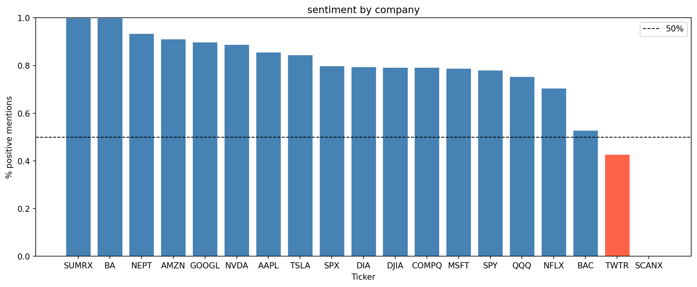
What do you notice about the sentiment distribution across companies? Do some companies have more positive sentiment than others? Can you think of any reasons why that might be the case?
Does social media sentiment track stock performance?
Naturally, an important question we’d want to ask is if positive social media coverage correlates with better stock performance. For this, we’ll get 3-month stock returns for our tickers using the yfinance package and compare them to their sentiment.
| ticker | pct_positive | total_mentions | return_3m | |
|---|---|---|---|---|
| 0 | BA | 1.000000 | 56 | -13.710716 |
| 1 | AMZN | 0.911765 | 110 | 6.393184 |
| 2 | GOOGL | 0.900000 | 44 | 9.709771 |
| 3 | NVDA | 0.888889 | 52 | 33.562053 |
| 4 | AAPL | 0.857143 | 81 | 30.551071 |
| 5 | TSLA | 0.846154 | 157 | 72.167558 |
| 6 | DIA | 0.795455 | 99 | 6.289547 |
| 7 | MSFT | 0.789474 | 48 | 13.735338 |
| 8 | SPY | 0.781513 | 301 | 8.723477 |
| 9 | QQQ | 0.754098 | 177 | 12.637074 |
| 10 | NFLX | 0.705882 | 99 | 20.809365 |
| 11 | BAC | 0.529412 | 44 | 21.158410 |
| 12 | SCANX | 0.000000 | 51 | 0.474903 |
fig, ax = plt.subplots(figsize=(9, 6))
ax.scatter(plot_df["pct_positive"],
    plot_df["return_3m"],s=plot_df["total_mentions"] * 2,alpha=0.7,
    color="steelblue",edgecolors="white", linewidths=0.5)

for _, row in plot_df.iterrows():
    ax.annotate(
        row["ticker"],
        (row["pct_positive"], row["return_3m"]),
        textcoords="offset points", xytext=(5, 3), fontsize=9)

ax.axhline(0, color="gray", linestyle="--", linewidth=0.8)
ax.axvline(0.5, color="gray", linestyle="--", linewidth=0.8)
ax.set_xlabel("% Positive Social Media Mentions")
ax.set_ylabel("3-Month Stock Return")
ax.set_title("Sentiment vs. 3-Month Stock Return")

corr = plot_df["pct_positive"].corr(plot_df["return_3m"])

plt.tight_layout()
plt.show() 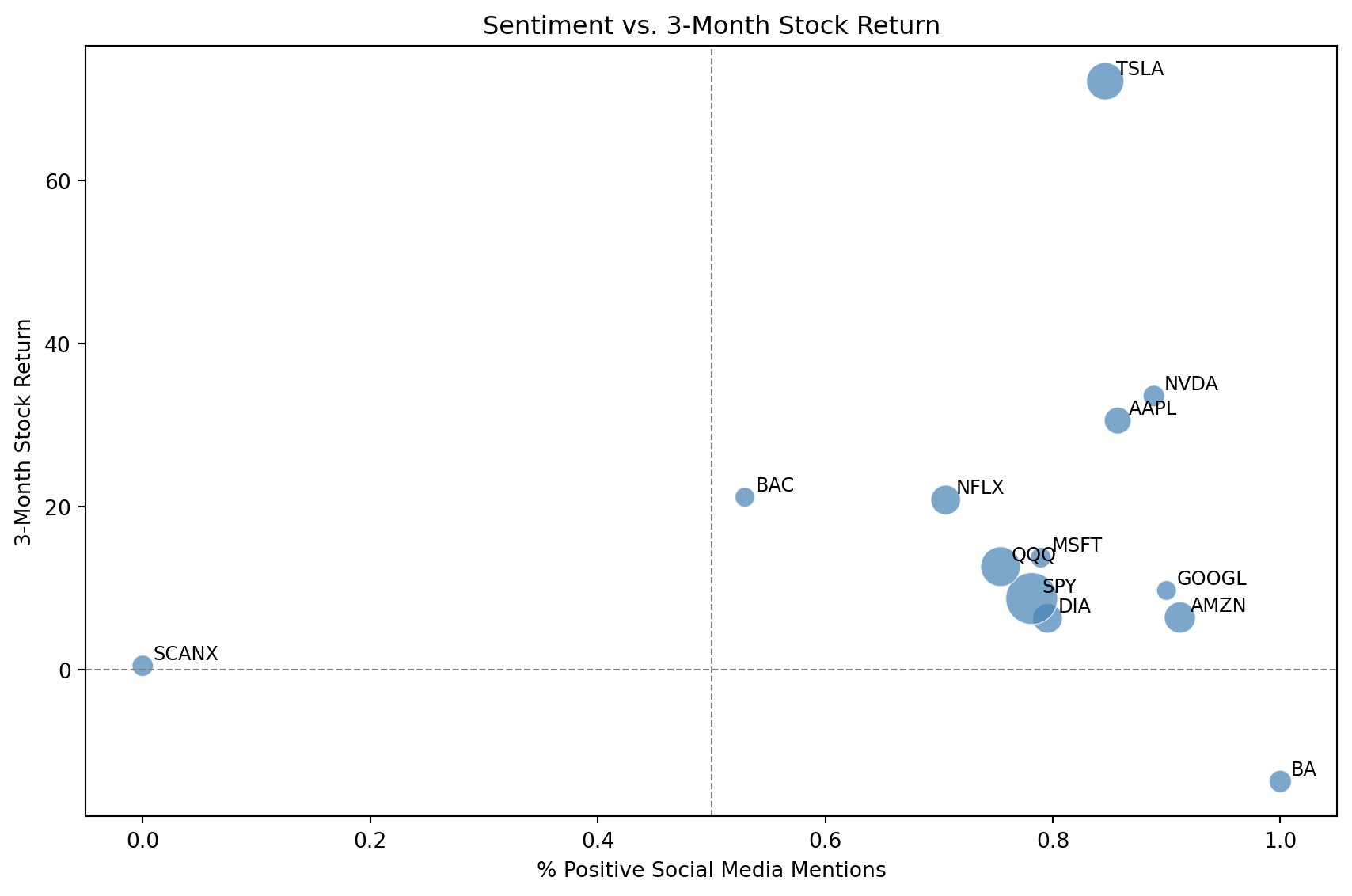
The scatterplot above shows a correlation between sentiment and returns. But correlation is not prediction. Can we actually use sentiment, combined with a company’s past performance, to forecast what will happen next? This might make us a lot of money if it works, but it’s also a much harder task. Let’s see how we might approach this problem.
We’ll model this using a simple linear regression:
\[ \hat y = \beta_0 + \beta_1 \cdot \text{sentiment score} + \beta_2 \cdot \text{past 1 month return} \]
This kind of mirrors the core idea from section 1. The model looks at what is known (sentiment and recent momentum of each stock ticker) and assigns weights to produce a prediction. The “vocabulary” here is just two features instead of thousands of words.
model_df = pd.merge(plot_df, past_returns_df, on="ticker").dropna()

X = model_df[["pct_positive", "past_1m_return"]].values
y = model_df["return_3m"].values

reg = LinearRegression()
reg.fit(X, y)


model_df["predicted_return"] = reg.predict(X)

print(f"Sentiment coefficient: {reg.coef_[0]:.2f}")
print(f"Past 1-month return coeff: {reg.coef_[1]:.2f}")
print(f"R^2: {reg.score(X, y):.3f}")
Sentiment coefficient: 8.86
Past 1-month return coeff: 1.15
R^2: 0.088fig, ax = plt.subplots(figsize=(7, 6))
ax.scatter(
model_df["return_3m"], model_df["predicted_return"], # y hat on y axis, y on x
color="steelblue", alpha=0.7, edgecolors="white", s=70
)
for _, row in model_df.iterrows():
ax.annotate(row["ticker"],
(row["return_3m"], row["predicted_return"]),
textcoords="offset points", xytext=(5, 3), fontsize=8)
lims = [min(model_df["return_3m"].min(), model_df["predicted_return"].min()) - 3,
max(model_df["return_3m"].max(), model_df["predicted_return"].max()) + 3,]
ax.plot(lims, lims, "k--", linewidth=0.8, label="Perfect prediction")
ax.set_xlabel("Actual 3-Month Return")
ax.set_ylabel("Predicted 3-Month Return")
ax.set_title("Predicted vs. Actual Returns")
ax.legend()
plt.tight_layout()
plt.show()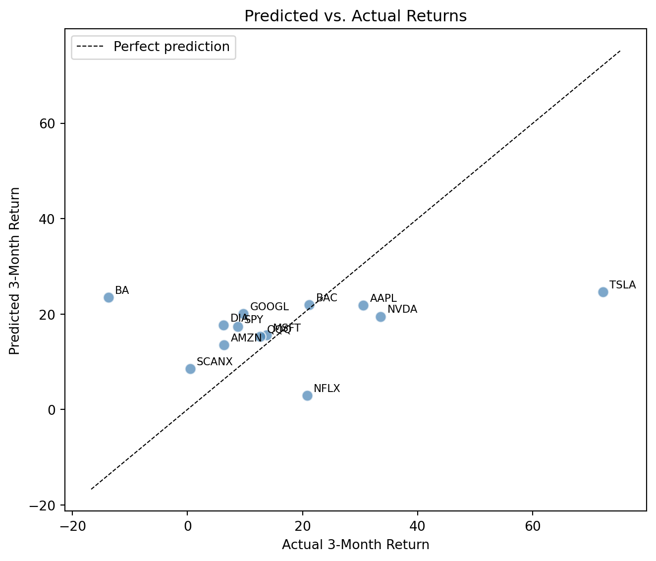
Points close to the dashed line are well predicted, while points far from it are errors. Based on the coefficients, does sentiment or short-term past returns have a stronger effect? This model was fit and evaluated on the same data. Why is in-sample \(R^2\) an optimistic measure of how well our model is performing? What would a proper evaluation require?
Think about the following: does a strong correlation here mean social media drives stock prices, or the other way around? What would you need to do, or could do, to make a causal claim?
Conclusion
This notebook showed how large language models process and make predictions about text, and how those predictions, which are grounded in probability distributions, can be applied to real financial data.
Key Takeaways
- Large language models (LLMs) predict the next word in a sequence by learning the probability distribution of possible outcomes based on context.
- LLMs can also be used to predict future values in a time series, such as stock prices, by incorporating additional features like public sentiment.
- Temperature controls how sharp or flat that distribution is, affecting how decisive or creative the model’s outputs are.
- Confidence scores are informative: a model’s probability for its top prediction correlates with its accuracy, making it a useful signal of reliability.
Glossary
- Large Language Model (LLM): A type of AI model that predicts the next word in a sequence based on the context of previous words.
- Token: A chunk of text the model processes: typically a word, part of a word, or punctuation. The phrase “the cat” might be split into two or three tokens depending on the model.
- Tokenizer: The component that splits raw text into tokens before the model sees it. Different models use different tokenizers, which is why the same sentence can produce different token counts.
- Word embedding: A list of numbers (a vector) representing a word’s meaning. Words used in similar contexts end up with similar vectors, so “profit” and “earnings” are close while “profit” and “elephant” are far apart. This is what lets a model relate words to each other.
- Next Word Prediction: The task of predicting the next word in a sequence given the previous words.
- Logits: The raw output scores a model produces for every possible next token, before they’re converted into probabilities. They can be any real number, positive or negative.
- Softmax: A function that converts logits into a valid probability distribution — every score becomes a number between 0 and 1, and they all sum to 1.
- Temperature: A knob that flattens or sharpens the probability distribution before the model picks a token. Low temperatures make the model pick the most likely word almost every time; high temperatures spread probability across more options, producing more varied outputs.
- Pretrained model: A model that has already been trained on a large dataset and saved, so you can use it directly without retraining. We use pretrained models in this notebook because training one from scratch would take enormous data and compute.
- Hugging Face: A popular platform that hosts and distributes pretrained ML models, including the ones used in this notebook. Think of it as a public library for models.
- RoBERTa: The specific pretrained model we use for sentiment classification (short for Robustly Optimized BERT Pretraining Approach). It reads the words before and after each target word, which helps it pick up on context and tone.
- Sentiment Analysis: The process of determining the emotional tone behind a series of words, used to understand the sentiment expressed in text.
- Confidence Score: The probability a model assigns to its top prediction; higher confidence correlates with higher accuracy on average.
- Confusion Matrix: A table that shows how often a classifier’s predictions agree or disagree with ground-truth labels, broken down by class.
References
- Kirsch, N. (2024, April 29). 10 Best AI Stocks Of August 2024. Forbes Advisor. https://www.forbes.com/advisor/investing/best-ai-stocks/
- Chen, J. (2023, October 6). Efficient Market Hypothesis (EMH): Forms and criticisms. Investopedia. https://www.investopedia.com/terms/e/efficientmarkethypothesis.asp
- Yahoo Finance. (n.d.). Yahoo Finance — Stocks, financial news, quotes, and market data. Retrieved August 1, 2025, from https://ca.finance.yahoo.com/
- Aroussi, R. (n.d.). yfinance [Python package]. GitHub. Retrieved August 1, 2025, from https://github.com/ranaroussi/yfinance
- Li, T. (2025). finvizfinance (Version 1.1.1) [Python package]. PyPI. Retrieved August 1, 2025, from https://pypi.org/project/finvizfinance/
- GeeksforGeeks. (2023, September 27). Complete guide to SARIMAX in Python. https://www.geeksforgeeks.org/python/complete-guide-to-sarimax-in-python/
- Sprenger, T. O., Tumasjan, A., Sandner, P. G., & Welpe, I. M. (2014, February 5). Twitter sentiment and stock market movements: The predictive power of social media. VoxEU. https://cepr.org/voxeu/columns/twitter-sentiment-and-stock-market-movements-predictive-power-social-media
- Wolf, T., Debut, L., Sanh, V., Chaumond, J., Delangue, C., Moi, A., … Rush, A. M. (2020). Transformers: State-of-the-art natural language processing. Proceedings of the 2020 Conference on Empirical Methods in Natural Language Processing: System Demonstrations, 38–45. https://huggingface.co/transformers/
- Sanh, V., Debut, L., Chaumond, J., & Wolf, T. (2019). DistilGPT2 [Pretrained language model]. Hugging Face. https://huggingface.co/distilbert/distilgpt2
- Paszke, A., Gross, S., Massa, F., Lerer, A., Bradbury, J., Chanan, G., … Chintala, S. (2019). PyTorch: An imperative style, high-performance deep learning library. Advances in Neural Information Processing Systems, 32. https://pytorch.org/