Learning Agents and Algorithmic Collusion

Python

game theory

reinforcement learning

Q-learning

The fourth and final notebook in the Game Theory stream. Two independent Q-learning agents play the pricing game from Notebook 1 over and over, with no communication and no model of each other, and teach themselves to hold prices above the one-shot Nash equilibrium, complete with punishment strategies. A small-scale replication of Calvano et al. (2020).

Author

Alex Ronczewski

Published

16 July 2026

Outline

Prerequisites

Notebook 3 of this stream, which builds on Notebooks 1 and 2: the pricing game, strategies as rules over history.
Basic Python and numpy at the COMET-intermediate level.
No reinforcement-learning background is needed: Q-learning is built from scratch here.

Learning Outcomes

By the end of this notebook you will be able to:

Describe Q-learning: states, actions, rewards, the Q-table, and the update rule.
Explain the two dials that make it work: the discount factor \(\delta\), equivalent to Notebook 3’s patience, and decaying \(\varepsilon\)-greedy exploration.
Train two independent Q-learners in the repeated pricing game and measure their profit gain over the one-shot Nash equilibrium.
Read a learned Q-table as a strategy (a rule over history).
Test that strategy with a forced price cut and recognize the learned punishment that sustains collusion.
Explain why algorithmic tacit collusion is hard to prosecute under competition law built around agreements.

import numpy as np
import matplotlib.pyplot as plt

RANDOM_STATE = 42  # fix randomness so the training runs are reproducible

1. Nobody writes the rules this time

Every player in this stream so far was given its behaviour in the form of a set algorithm. Notebook 1 solved the three-price game by iterated elimination: rational one-shot firms post Medium and earn 30 a day. Notebook 3 repeated the game and showed that hand-written rules like grim trigger can hold prices at High, awarding profits of 50 a day, and the folk theorem said a whole continuum of outcomes is sustainable.

This notebook removes the humans entirely. Each firm’s pricing is handed to a Q-learning agent, one of the standard reinforcement-learning algorithms and a small cousin of the methods behind game-playing AI systems. Each agent observes yesterday’s two prices and its own profit, and nothing else. It is not told the payoff table, it is not told that a rival exists. The two agents share no code and never communicate. We then answer the main question of this stream: what do they converge to? This experiment is a small-scale replication of Calvano, Calzolari, Denicolo, and Pastorello (2020).

The market is Notebook 1’s three-price game, with the benchmarks we have already computed: the one-shot Nash equilibrium (Medium, Medium) pays 30 to each firm, and the collusive outcome (High, High) pays 50.

A3 = np.array([[50, 20, 20],
               [60, 30, 12],
               [20, 20, 10]])   # rows and columns: High, Medium, Low
prices = ["High", "Medium", "Low"]

NASH, COLLUSION = 30, 50

2. Q-learning in one table

An agent’s world has three parts. The state \(s\) is what it sees before acting: yesterday’s pair of prices, mine and the rival’s, so there are \(3 \times 3 = 9\) total states. The action \(a\) is today’s price, and the reward is today’s profit.

The agent’s entire brain is a table of 27 numbers: \(Q(s, a)\) estimates the total discounted profit from taking action \(a\) in state \(s\) and behaving logically afterwards. After every day it nudges one entry toward what it just experienced:

\[ Q(s, a) \leftarrow (1 - \alpha)\, Q(s, a) + \alpha \left[ \text{profit} + \delta \max_{a'} Q(s', a') \right]. \]

The learning rate \(\alpha\) sets how fast new experience overwrites old beliefs. The discount factor \(\delta\) weights the future: the term \(\delta \max_{a'} Q(s', a')\) is the value of the state the action led to, so an action is credited with the profits it opens up tomorrow, shrunk by \(\delta\). This is the same \(\delta\) as Notebook 3’s continuation probability, and we set it to 0.95: it sits comfortably above every collusion threshold we derived. Notice what the update does not contain: no belief about the opponent, no model of the game. Where Notebook 2’s fictitious play predicted the rival and best responded, Q-learning just scores its own actions by results and does not think about the rival.

The last ingredient is exploration. An agent that always plays its current best guess can never discover a better one, so with probability \(\varepsilon\) it picks a random price instead, and \(\varepsilon\) decays over training: try everything early, exploit what you learned late.

def run_session(rng, steps, alpha=0.15, delta=0.95, beta=4.5e-5):
    Q = [rng.uniform(0, 1, (9, 3)), rng.uniform(0, 1, (9, 3))]
    a = [int(rng.integers(3)), int(rng.integers(3))]
    profits = np.empty((steps, 2))
    for t in range(steps):
        s = (3 * a[0] + a[1], 3 * a[1] + a[0])     # each agent: (my last price, rival's last price)
        eps = np.exp(-beta * t)                    # exploration fades as training goes on
        for i in range(2):
            if rng.random() < eps:
                a[i] = int(rng.integers(3))
            else:
                a[i] = int(np.argmax(Q[i][s[i]]))
        r = (A3[a[0], a[1]], A3[a[1], a[0]])
        s2 = (3 * a[0] + a[1], 3 * a[1] + a[0])
        for i in range(2):
            Q[i][s[i], a[i]] += alpha * (r[i] + delta * Q[i][s2[i]].max() - Q[i][s[i], a[i]])
        profits[t] = r
    return Q, profits, a

3. Prices climb past Nash

We train 20 independent pairs of agents, 100,000 days each. Every session starts from scratch: fresh random Q-tables, no memory of the other sessions.

This training cell is the most computationally intensive of the stream and will take longer to run (~1 minute depending on hardware).

rng = np.random.default_rng(RANDOM_STATE)
sessions = [run_session(rng, 100_000) for _ in range(20)]

final = np.array([p[-5000:].mean() for _, p, _ in sessions])
gain = (final.mean() - NASH) / (COLLUSION - NASH)
print(f"mean profit over the last 5,000 days, averaged across sessions: {final.mean():.1f}")
print(f"one-shot Nash pays {NASH}, full collusion pays {COLLUSION}")
print(f"profit gain captured: {gain:.0%} of the way from Nash to collusion")

mean profit over the last 5,000 days, averaged across sessions: 48.6
one-shot Nash pays 30, full collusion pays 50
profit gain captured: 93% of the way from Nash to collusion

window = np.ones(2000) / 2000
xs = np.arange(2000 - 1, 100_000)[::200]

plt.figure(figsize=(9, 5))
curves = []
for _, profits, _ in sessions:
    smooth = np.convolve(profits.mean(axis=1), window, mode="valid")
    curves.append(smooth)
    plt.plot(xs, smooth[::200], color="grey", alpha=0.25, linewidth=1)
plt.plot(xs, np.mean(curves, axis=0)[::200], color="tab:blue", linewidth=2,
         label="average of 20 sessions")
plt.axhline(COLLUSION, color="black", linestyle="--", linewidth=1, label="full collusion (50)")
plt.axhline(NASH, color="black", linestyle=":", linewidth=1, label="one-shot Nash (30)")
plt.xlabel("day of training")
plt.ylabel("profit per firm per day (rolling average)")
plt.title("Twenty pairs of independent Q-learners price their way past Nash")
plt.legend(loc="lower right")
plt.show()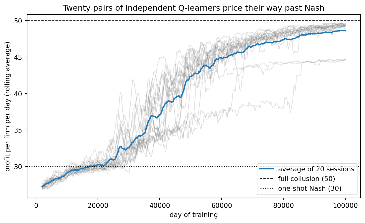

Early on, while the agents explore at random, profits sit slightly below 30 (Nash Payoff). As exploration fades, every session climbs, and continues past 30. The average settles near 49, about 93% of the distance from the competitive benchmark to full collusion. No economist told these agents that (High, High) was worth aiming for. Two profit-maximizing algorithms, each treating the other as background noise, found the collusive outcome on their own.

4. The strategy they invented

Where exactly did each session land? We freeze the learned Q-tables, switch off exploration, and let each pair play greedily until its behaviour repeats.

def greedy_path(Qs, a, periods, force=None):
    path = []
    for t in range(periods):
        s = (3 * a[0] + a[1], 3 * a[1] + a[0])
        a = [int(np.argmax(Qs[0][s[0]])), int(np.argmax(Qs[1][s[1]]))]
        if force is not None and t == force[0]:
            a[force[1]] = force[2]
        path.append(tuple(a))
    return path

tails = [greedy_path(Q, a, 60)[-20:] for Q, _, a in sessions]
n_collusive = sum(all(step == (0, 0) for step in tail) for tail in tails)
print(f"{n_collusive} of 20 sessions settle at constant (High, High)")
print(f"the other {20 - n_collusive} settle into two-day cycles that include (High, High)")

17 of 20 sessions settle at constant (High, High)
the other 3 settle into two-day cycles that include (High, High)

Seventeen sessions sit permanently at (High, High). The remaining three cycle between (High, High) and a one-sided undercut, averaging above Nash as well. But a price is only half the story: Notebook 3 taught us that collusion is sustained by what would happen after a deviation. The agents’ contingency plans are sitting in their Q-tables, and we can read one out as a rule over history, just like the strategies of Notebook 3:

Q_example = next(Q for (Q, _, a), tail in zip(sessions, tails)
                 if all(step == (0, 0) for step in tail))[0]

print("learned greedy rule (rows: my last price, columns: rival's last price)")
print(f"{'':14}" + "".join(f"rival {p:8}" for p in prices))
for mine in range(3):
    row = [prices[int(np.argmax(Q_example[3 * mine + theirs]))] for theirs in range(3)]
    print(f"I was {prices[mine]:8}" + "".join(f"{p:14}" for p in row))

learned greedy rule (rows: my last price, columns: rival's last price)
              rival High    rival Medium  rival Low     
I was High    High          Medium        High          
I was Medium  Medium        High          Medium        
I was Low     Medium        High          High

The top-left corner of the table is the part that actual play visits. If both firms priced High yesterday, price High again. If I was High and the rival undercut to Medium, drop to Medium: punish. And once both of us are at Medium, go back to High: forgive. That is a one-day trigger strategy with built-in forgiveness, a close cousin of win-stay-lose-shift, except nobody sent it in, wrote it, or programmed it. It was created out of profit feedback.

If the punishment is real, it should show up in behaviour. We run Calvano et al.’s signature test on the 17 collusive sessions: let play settle at (High, High), then force firm 1 to undercut to Medium for a single day, and watch both agents play greedily afterwards.

episodes = np.array([greedy_path(Q, [0, 0], 12, force=(3, 0, 1))
                     for (Q, _, _), tail in zip(sessions, tails)
                     if all(step == (0, 0) for step in tail)])

labels = [f"({prices[i]}, {prices[j]})" for i, j in episodes[0]]
print("one session's episode:", " -> ".join(labels[2:8]))

plt.figure(figsize=(9, 4.5))
plt.plot(episodes[:, :, 0].mean(axis=0), color="tab:red", marker="o", label="firm 1 (forced to undercut)")
plt.plot(episodes[:, :, 1].mean(axis=0), color="tab:blue", marker="o", label="firm 2 (its rival)")
plt.axvline(3, color="black", linestyle="--", linewidth=1, label="forced undercut")
plt.yticks([0, 1, 2], prices)
plt.ylim(2.2, -0.2)
plt.xlabel("day")
plt.ylabel("price posted (average over 17 sessions)")
plt.title("One forced undercut: punished the next day, forgiven the day after")
plt.legend(loc="center right")
plt.show()

one session's episode: (High, High) -> (Medium, High) -> (Medium, Medium) -> (High, High) -> (High, High) -> (High, High)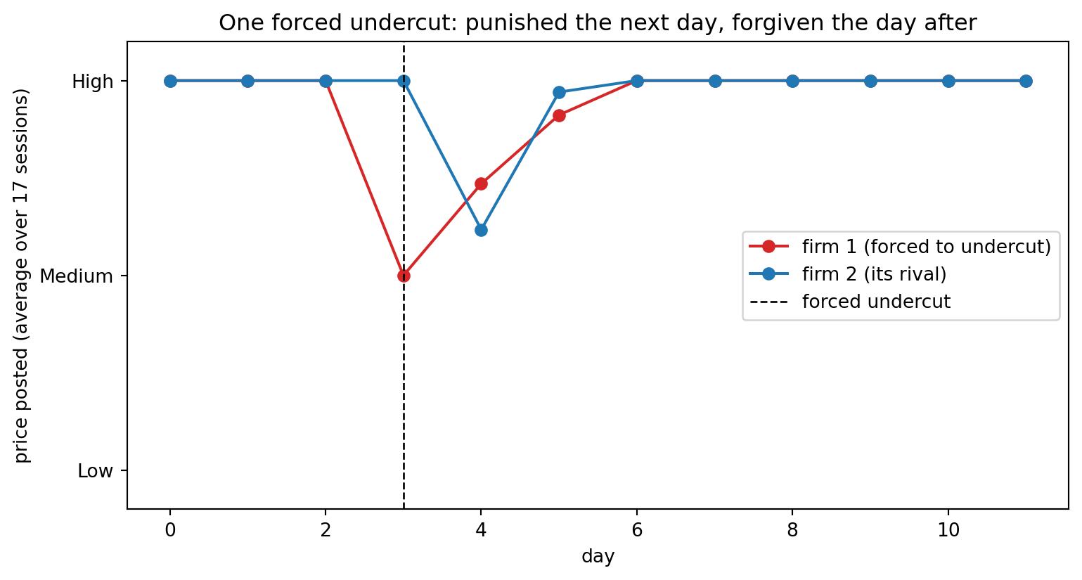

In most sessions the rival answers the undercut with a price cut of its own on the very next day, and every session is back at (High, High) within three days of the shock. Check the deviator’s arithmetic: the undercut earned 60 instead of 50 on the day, then the punishment round paid around 30 instead of 50. The one-day gain of 10 buys a next-day loss of 20. The agents learned a retaliation scheme that makes undercutting a losing move, which is precisely the incentive structure Notebook 3 said collusion requires.

5. Patience is the mechanism

Notebook 3’s theory says all of this should collapse if the future stops mattering. Q-learning gives us the dial directly: retrain the agents with \(\delta = 0\), so each action is credited only with the profit it earns today.

rng_myopic = np.random.default_rng(RANDOM_STATE)
myopic = [run_session(rng_myopic, 100_000, delta=0.0) for _ in range(5)]

final_myopic = np.array([p[-5000:].mean() for _, p, _ in myopic])
print(f"myopic agents' mean profit over the last 5,000 days: {final_myopic.mean():.1f}")

plt.figure(figsize=(9, 4.5))
plt.plot(xs, np.mean(curves, axis=0)[::200], color="tab:blue", linewidth=2,
         label="patient agents (delta = 0.95)")
myopic_mean = np.mean([np.convolve(p.mean(axis=1), window, mode="valid") for _, p, _ in myopic], axis=0)
plt.plot(xs, myopic_mean[::200], color="tab:red", linewidth=2, label="myopic agents (delta = 0)")
plt.axhline(COLLUSION, color="black", linestyle="--", linewidth=1)
plt.axhline(NASH, color="black", linestyle=":", linewidth=1)
plt.xlabel("day of training")
plt.ylabel("profit per firm per day (rolling average)")
plt.title("Take away the future and the agents find the one-shot Nash instead")
plt.legend(loc="lower right")
plt.show()

myopic agents' mean profit over the last 5,000 days: 30.0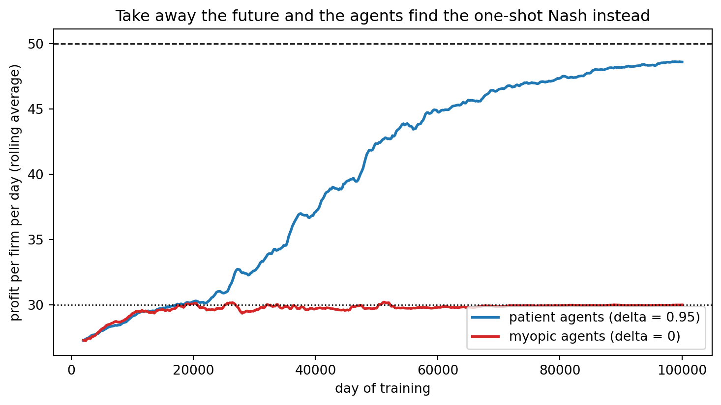

Myopic agents converge to a profit of 30: they learn the game perfectly well and play the strategy from Notebook 1 - the one-shot Nash equilibrium. Collusion is worthless to an agent that cannot value tomorrow, because sustaining it means passing up today’s undercut for the sake of future cooperation. The shadow of the future is the mechanism, just like theory predicted.

Self-test

Apply Notebook 3’s threshold formula to this game: deviating from (High, High) to Medium earns 60 once, and Nash-reversion punishment pays 30 forever after. How patient do the firms have to be for High prices to be sustainable, and do our two training runs sit on the sides of that threshold you would expect?

Show / hide answer

The threshold is \(\delta \ge (T - R)/(T - P) = (60 - 50)/(60 - 30) = 1/3\). Our patient agents have \(\delta = 0.95\), far above it, and collude; the myopic agents have \(\delta = 0\), far below it, and price at Nash. The Q-learners were never shown this formula, but their learned behaviour follows it. They learned it indirectly.

6. Where in the green region, and why regulators care

Notebook 3 ended with the folk theorem: for this game, every average payoff pair above the guaranteed minimum is an equilibrium of the repeated game, and theory cannot say which one will occur. We closed by promising to watch which point the learning algorithms find. Here is the answer: each dot is one training session’s long-run average payoff pair.

pairs = np.array([np.mean([[A3[i, j], A3[j, i]] for i, j in tail], axis=0) for tail in tails])

feasible = plt.Polygon([(10, 10), (60, 20), (50, 50), (20, 60)], closed=True,
                       color="tab:blue", alpha=0.12, label="feasible average payoffs")
sustainable = plt.Polygon([(20, 20), (60, 20), (50, 50), (20, 60)], closed=True,
                          color="tab:green", alpha=0.30, label="equilibria of the repeated game")

fig, ax = plt.subplots(figsize=(7, 6.5))
ax.add_patch(feasible)
ax.add_patch(sustainable)
ax.scatter(pairs[:, 0], pairs[:, 1], color="black", zorder=3, s=30, label="where the 20 sessions landed")
ax.annotate(f"{n_collusive} sessions", (50, 50), textcoords="offset points", xytext=(8, 2))
ax.scatter(30, 30, color="tab:red", zorder=3, s=30)
ax.annotate("one-shot Nash", (30, 30), textcoords="offset points", xytext=(8, -4))
ax.set_xlim(0, 68)
ax.set_ylim(0, 68)
ax.set_xlabel("firm 1's average profit per day")
ax.set_ylabel("firm 2's average profit per day")
ax.set_title("The folk theorem's green region, and where learning actually lands")
ax.legend(loc="lower left")
plt.show()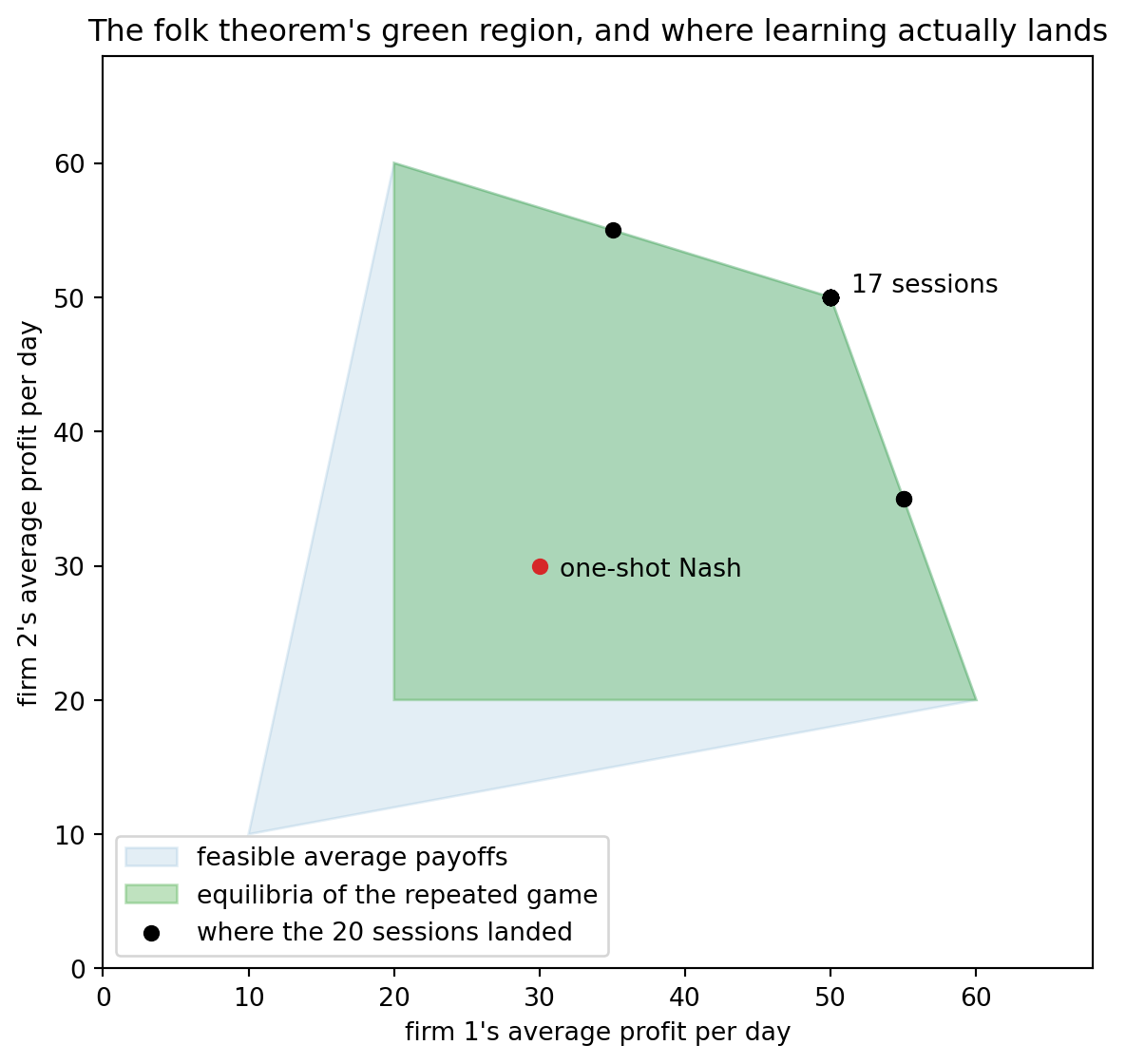

The sessions pile up at full collusion, with a few landing on nearby asymmetric cycles, and none at the competitive corner. Out of a continuum of stable outcomes, independent learning selected the most profitable one for the firms, at their customers’ expense.

That is why this experiment, and the Calvano et al. paper behind it, attracted regulators’ attention. Real evidence points to the same thing: when algorithmic pricing software spread through the German retail gasoline market, margins rose noticeably in the markets where competing stations had both adopted it (Assad et al., 2024). And the legal problem is structural.

There is no agreement to prosecute

Cartel law is built around agreement: messages, meetings, a concerted practice that investigators can subpoena. Here there is nothing to find. The two agents never communicated, were never told a rival existed, and each independently maximized its own profit, which is exactly what firms are expected to do. The supra-competitive prices and the punishment threat that sustains them live in two tables of 27 numbers (many more in this case) that even the firms’ own engineers may never have inspected. The outcome is collusive in every economic sense, yet involves no legal agreement, and how to regulate that gap, auditing pricing algorithms, testing them in sandboxes before deployment, or holding firms liable for what their software converges to, is an open policy question.

7. Conclusion

This is the last notebook, so let us look back at the whole stream. Notebook 1 asked what rational players would do and answered with equilibrium: in the three-price game, Medium, a payoff of 30. Notebook 2 replaced reasoning with belief-based learning and found that play can converge to equilibria, select among them, or cycle forever. Notebook 3 repeated the game and showed that history-dependent rules sustain cooperation, at a continuum of possible outcomes from the folk theorem. And here, two Q-learners that know nothing of equilibria, thresholds, or each other worked their way to the collusive corner of that outcome set and invented the punishment strategies that keep it stable, provided only that they valued the future.

The stream’s two questions now have their answers. What is the equilibrium? Can be all kinds of things. What do interacting algorithms converge to? Something specific, discoverable by simulation, and sometimes alarmingly: the players of the algorithmic economy do find the equilibria of game theory, including the ones consumers would rather they wouldn’t.

Thank you for reading!

7.1 Where to go next

Everything in this stream happened in simultaneous-move games with a handful of actions.

Sequential and extensive-form games. In many markets one player moves first and the other observes before responding: a leader posts a price, an entrant decides whether to challenge an incumbent. Game trees, backward induction, and subgame perfect equilibira: this is the other half of ECON 421.
Auctions and games of incomplete information. Every game here was played with both payoff tables on the table. Auction theory drops that assumption, each bidder knows only its own valuation, and it is where algorithmic players are most common in practice: every search ad you see was sold in an auction among bidding bots, run billions of times a day.
Multi-agent reinforcement learning at scale. Notebook 4’s agents fit in a table of 27 numbers. Replace the table with a neural network (this prAxIs notebook introduces them) and the same learning loop scales to games far too large to tabulate, which is how self-play systems reached superhuman Go and poker.

7.2 Recommended reading

Osborne, An Introduction to Game Theory (Oxford University Press). The standard undergraduate text, and the closest match to ECON 421.
Shoham and Leyton-Brown, Multiagent Systems: Algorithmic, Game-Theoretic, and Logical Foundations (masfoundations.org). Free online, covers the computer science side of everything in this stream, and one of its authors teaches at UBC.
Axelrod, The Evolution of Cooperation (Basic Books). The story behind Notebook 3’s tournament, written for a general audience and still the best account of why nice strategies win.
The nashpy (nashpy.readthedocs.io) and axelrod (axelrod.readthedocs.io) documentation. Both go well beyond what we used, and the axelrod library ships over 200 strategies you can drop into Notebook 3’s tournament.

References

Assad, S., Clark, R., Ershov, D., & Xu, L. (2024). Algorithmic pricing and competition: Empirical evidence from the German retail gasoline market. Journal of Political Economy, 132(3), 723-771. The field evidence of section 6.
Calvano, E., Calzolari, G., Denicolo, V., & Pastorello, S. (2020). Artificial intelligence, algorithmic pricing, and collusion. American Economic Review, 110(10), 3267-3297. The experiment this notebook replicates at small scale.
Klein, T. (2021). Autonomous algorithmic collusion: Q-learning under sequential pricing. RAND Journal of Economics, 52(3), 538-558. A companion result with firms moving in turns.
Li, H. ECON 221 and ECON 421 course outlines. University of British Columbia. https://lihao.microeconomics.ca/li_content/econ421/outline.html
OECD (2017). Algorithms and collusion: Competition policy in the digital age. OECD roundtable report. https://www.oecd.org/competition/algorithms-collusion-competition-policy-in-the-digital-age.htm
Sutton, R. S., & Barto, A. G. (2020). Reinforcement Learning: An Introduction (2nd ed.). MIT Press. http://incompleteideas.net/book/RLbook2020.pdf (Chapter 6 covers Q-learning.)
Watkins, C. J. C. H., & Dayan, P. (1992). Q-learning. Machine Learning, 8, 279-292. The algorithm itself.