Double / Debiased Machine Learning

ECON526

Paul Schrimpf

University of British Columbia

Table of contents

• Introduction
• Theory
• Creating Orthogonal Moments
• Example: Gender Wage Gap

Introduction

\[ \def\indep{\perp\!\!\!\perp} \def\Er{\mathrm{E}} \def\R{\mathbb{R}} \def\En{{\mathbb{E}_n}} \def\Pr{\mathrm{P}} \newcommand{\norm}[1]{\left\Vert {#1} \right\Vert} \newcommand{\abs}[1]{\left\vert {#1} \right\vert} \def\inprob{{\,{\buildrel p \over \rightarrow}\,}} \def\indist{\,{\buildrel d \over \rightarrow}\,} \DeclareMathOperator*{\plim}{plim} \DeclareMathOperator*{\argmax}{arg\,max} \DeclareMathOperator*{\argmin}{arg\,min} \]

Introduction

• Many estimation tasks involve:
  • Low dimensional parameter of interest
  • High dimensional nuisance parameters needed to recover parameter of interest
• Example: in matching
  • Interested in \(ATE = \Er[Y(1) - Y(0)]\)
  • Nuisance parameters \(\Er[Y|D,X]\) and/or \(P(D=1|X)\)

Machine Learning for Nuisance Parameters

• In matching we said that we could use flexible machine learning estimators for \(\Er[Y|D,X]\) and \(P(D=1|X)\) and plug them into the doubly robust estimator

• We will cover:

  • Some of the technical details behind this idea
  • How this idea can be applied to other estimators

These notes will examine the incorportion of machine learning methods in classic econometric techniques for estimating causal effects. More specifally, we will focus on estimating treatment effects using matching and instrumental variables. In these estimators (and many others) there is a low-dimensional parameter of interest, such as the average treatment effect, but estimating it requires also estimating a potentially high dimensional nuisance parameter, such as the propensity score. Machine learning methods were developed for prediction with high dimensional data. It is then natural to try to use machine learning for estimating high dimensional nuisance parameters. Care must be taken when doing so though because the flexibility and complexity that make machine learning so good at prediction also pose challenges for inference.

Example: partially linear model

\[ y_i = \theta d_i + f(x_i) + \epsilon_i \]

• Interested in \(\theta\)
• Assume \(\Er[\epsilon|d,x] = 0\)
• Nuisance parameter \(f()\)

Example: Matching

• Binary treatment \(d_i \in \{0,1\}\)
• Potential outcomes \(y_i(0), y_i(1)\), observe \(y_i = y_i(d_i)\)
• Interested in average treatment effect : \(\theta = \Er[y_i(1) - y_i(0)]\)
• Covariates \(x_i\)
• Assume unconfoundedness : \(d_i \indep y_i(1), y_i(0) | x_i\)

The partially linear and matching models are closely related. If the conditional mean independence assumption of the partially linear model is strengthing to conditional indepence then the partially linear model is a special case of the matching model with constant treatment effects, \(y_i(1) - y_i(0) = \theta\). Thus the matching model can be viewed as a generalization of the partially linear model that allows for treatment effect heterogeneity.

Example: Matching

• Estimatable formulae for ATE : \[ \begin{align*} \theta = & \Er\left[\frac{y_i d_i}{\Pr(d = 1 | x_i)} - \frac{y_i (1-d_i)}{1-\Pr(d=1|x_i)} \right] \\ \theta = & \Er\left[\Er[y_i | d_i = 1, x_i] - \Er[y_i | d_i = 0 , x_i]\right] \\ \theta = & \Er\left[ \begin{array}{l} d_i \frac{y_i - \Er[y_i | d_i = 1, x_i]}{\Pr(d=1|x_i)} - (1-d_i)\frac{y_i - \Er[y_i | d_i = 0, x_i]}{1-\Pr(d=1|x_i)} + \\ + \Er[y_i | d_i = 1, x_i] - \Er[y_i | d_i = 0 , x_i]\end{array}\right] \end{align*} \]

Example: IV

\[ \begin{align*} y_i = & \theta d_i + f(x_i) + \epsilon_i \\ d_i = & g(x_i, z_i) + u_i \end{align*} \]

• Interested in \(\theta\)
• Assume \(\Er[\epsilon|x,z] = 0\), \(\Er[u|x,z]=0\)
• Nuisance parameters \(f()\), \(g()\)

Example: LATE

• Binary instrumet \(z_i \in \{0,1\}\)
• Potential treatments \(d_i(0), d_i(1) \in \{0,1\}\), \(d_i = d_i(Z_i)\)
• Potential outcomes \(y_i(0), y_i(1)\), observe \(y_i = y_i(d_i)\)
• Covariates \(x_i\)
• \((y_i(1), y_i(0), d_i(1), d_i(0)) \indep z_i | x_i\)
• Local average treatment effect: \[ \begin{align*} \theta = & \Er\left[\Er[y_i(1) - y_i(0) | x, d_i(1) > d_i(0)]\right] \\ = & \Er\left[\frac{\Er[y|z=1,x] - \Er[y|z=0,x]} {\Er[d|z=1,x]-\Er[d|z=0,x]} \right] \end{align*} \]

Theory

General setup

• Parameter of interest \(\theta \in \R^{d_\theta}\)

• Nuisance parameter \(\eta \in T\)

• Moment conditions \[ \Er[\psi(W;\theta_0,\eta_0) ] = 0 \in \R^{d_\theta} \] with \(\psi\) known

• Estimate \(\hat{\eta}\) using some machine learning method

• Estimate \(\hat{\theta}\) from \[ \En[\psi(w_i;\hat{\theta},\hat{\eta}) ] = 0 \]

We are following the setup and notation of Chernozhukov et al. (2018). As in the examples, the dimension of \(\theta\) is fixed and small. The dimension of \(\eta\) is large and might be increasing with sample size. \(T\) is some normed vector space.

Example: partially linear model

\[ y_i = \theta_0 d_i + f_0(x_i) + \epsilon_i \]

• Compare the estimates from

  1. \(\En[d_i(y_i - \tilde{\theta} d_i - \hat{f}(x_i)) ] = 0\)

  and

  2. \(\En[(d_i - \hat{m}(x_i))(y_i - \hat{\mu}(x_i) - \theta (d_i - \hat{m}(x_i)))] = 0\)

  where \(m(x) = \Er[d|x]\) and \(\mu(y) = \Er[y|x]\)

Example: partially linear model In the partially linear model,

\[ y_i = \theta_0 d_i + f_0(x_i) + \epsilon_i \]

we can let \(w_i = (y_i, x_i)\) and \(\eta = f\). There are a variety of candidates for \(\psi\). An obvious (but flawed) one is \(\psi(w_i; \theta, \eta) = (y_i - \theta_0 d_i - f_0(x_i))d_i\). With this choice of \(\psi\), we have

\[ \begin{align*} 0 = & \En[d_i(y_i - \hat{\theta} d_i - \hat{f}(x_i)) ] \\ \hat{\theta} = & \En[d_i^2]^{-1} \En[d_i (y_i - \hat{f}(x_i))] \\ (\hat{\theta} - \theta_0) = & \En[d_i^2]^{-1} \En[d_i \epsilon_i] + \En[d_i^2]^{-1} \En[d_i (f_0(x_i) - \hat{f}(x_i))] \end{align*} \]

The first term of this expression is quite promising. \(d_i\) and \(\epsilon_i\) are both finite dimensional random variables, so a law of large numbers will apply to \(\En[d_i^2]\), and a central limit theorem would apply to \(\sqrt{n} \En[d_i \epsilon_i]\). Unfortunately, the second expression is problematic. To accomodate high dimensional \(x\) and allow for flexible \(f()\), machine learning estimators must introduce some sort of regularization to control variance. This regularization also introduces some bias. The bias generally vanishes, but at a slower than \(\sqrt{n}\) rate. Hence

\[ \sqrt{n} \En[d_i (f_0(x_i) - \hat{f}(x_i))] \to \infty. \]

To get around this problem, we must modify our estimate of \(\theta\). Let \(m(x) = \Er[d|x]\) and \(\mu(y) = \Er[y|x]\). Let \(\hat{m}()\) and \(\hat{\mu}()\) be some estimates. Then we can estimate \(\theta\) by partialling out:

\[ \begin{align*} 0 = & \En[(d_i - \hat{m}(x_i))(y_i - \hat{\mu}(x_i) - \theta (d_i - \hat{m}(x_i)))] \\ \hat{\theta} = & \En[(d_i -\hat{m}(x_i))^2]^{-1} \En[(d_i - \hat{m}(x_i))(y_i - \hat{\mu}(x_i))] \\ (\hat{\theta} - \theta_0) = & \En[(d_i -\hat{m}(x_i))^2]^{-1} \left(\En[(d_i - \hat{m}(x_i))\epsilon_i] + \En[(d_i - \hat{m}(x_i))(\mu(x_i) - \hat{\mu}(x_i))] \right) \\ = & \En[(d_i -\hat{m}(x_i))^2]^{-1} \left( a + b +c + d \right) \end{align*} \]

where

\[ \begin{align*} a = & \En[(d_i -m(x_i))\epsilon_i] \\ b = & \En[(m(x_i)-\hat{m}(x_i))\epsilon_i] \\ c = & \En[v_i(\mu(x_i) - \hat{\mu}(x_i))] \\ d = & \En[(m(x_i) - \hat{m}(x_i))(\mu(x_i) - \hat{\mu}(x_i))] \end{align*} \]

with \(v_i = d_i - \Er[d_i | x_i]\). The term \(a\) is well behaved and \(\sqrt{n}a \leadsto N(0,\Sigma)\) under standard conditions. Although terms \(b\) and \(c\) appear similar to the problematic term in the initial estimator, they are better behaved because \(\Er[v|x] = 0\) and \(\Er[\epsilon|x] = 0\). This makes it possible, but difficult to show that \(\sqrt{n}b \to_p = 0\) and \(\sqrt{n} c \to_p = 0\), see e.g. Belloni, Chernozhukov, and Hansen (2014). However, the conditions on \(\hat{m}\) and \(\hat{\mu}\) needed to show this are slightly restrictive, and appropriate conditions might not be known for all estimators. Chernozhukov et al. (2018) describe a sample splitting modification to \(\hat{\theta}\) that allows \(\sqrt{n} b\) and \(\sqrt{n} c\) to vanish under weaker conditions (essentially the same rate condition as needed for \(\sqrt{n} d\) to vanish.)

The last term, \(d\), is a considerable improvement upon the first estimator. Instead of involving the error in one estimate, it now involes the product of the error in two estimates. By the Cauchy-Schwarz inequality, \[ d \leq \sqrt{\En[(m(x_i) - \hat{m}(x_i))^2]} \sqrt{\En[(\mu(x_i) - \hat{\mu}(x_i))^2]}. \] So if the estimates of \(m\) and \(\mu\) converge at rates faster than \(n^{-1/4}\), then \(\sqrt{n} d \to_p 0\). This \(n^{-1/4}\) rate is reached by many machine learning estimators.

Lessons from the example

• Need an extra condition on moments – Neyman orthogonality \[ \partial \eta \Er[\psi(W;\theta_0,\eta_0)](\eta-\eta_0) = 0 \]

• Want estimators faster than \(n^{-1/4}\) in the prediction norm, \[ \sqrt{\En[(\hat{\eta}(x_i) - \eta(x_i))^2]} \lesssim_P n^{-1/4} \]

• Also want estimators that satisfy something like \[ \sqrt{n} \En[(\eta(x_i)-\hat{\eta}(x_i))\epsilon_i] = o_p(1) \]

  • Sample splitting / cross-fitting will make this easier

Cross-fitting

• Randomly partition into \(K\) subsets \((I_k)_{k=1}^K\)
• \(I^c_k = \{1, ..., n\} \setminus I_k\)
• \(\hat{\eta}_k =\) estimate of \(\eta\) using \(I^c_k\)
• Estimator: \[ \begin{align*} 0 = & \frac{1}{K} \sum_{k=1}^K \frac{K}{n} \sum_{i \in I_k} \psi(w_i;\hat{\theta}^{DML},\hat{\eta}_k) \\ 0 = & \frac{1}{K} \sum_{k=1}^K \En_k[ \psi(w_i;\hat{\theta}^{DML},\hat{\eta}_k)] \end{align*} \]

Assumptions

1. Neyman Orthogonality \[ \partial \eta \Er[\psi(W;\theta_0,\eta_0)](\eta-\eta_0) \approx 0 \]
2. Fast enough convergence of \(\hat{\eta}\) \[ \sqrt{\Er[(\hat{\eta}_k(x_i) - \eta(x_i))^2|I_k^c]} \lesssim_P n^{-1/4} \]
3. Various moments exist and other regularity conditions
4. Moment condition linear in \(\theta\) (to simplify notation only) \[ \psi(w;\theta,\eta) = \psi^a(w;\eta) \theta + \psi^b(w;\eta) \]

¹

1. These are stated loosely, see Chernozhukov et al. (2018) for precise conditions.

Asymptotic Normality

\[ \sqrt{n} \sigma^{-1} (\hat{\theta} - \theta_0) = \frac{1}{\sqrt{n}} \sum_{i=1}^n \bar{\psi}(w_i) + o_p(1) \indist N(0,1) \] - Variance \[\sigma^2 = \Er[\psi^a(w_i;\eta_0)]^{-1} \Er\left[ \psi(w;\theta_0,\eta_0) \psi(w;\theta_0,\eta_0)'\right] \Er[\psi^a(w_i;\eta_0)]^{-1} \] - Influence function \[\bar{\psi}(w) = -\sigma^{-1} \Er[\psi^a(w_i;\eta_0)]^{-1} \psi(w;\theta_0,\eta_0)\]

Creating Orthogonal Moments

Creating orthogonal moments

• Need \[ \partial \eta\Er\left[\psi(W;\theta_0,\eta_0)[\eta-\eta_0] \right] \approx 0 \]

• Given an some model, how do we find a suitable \(\psi\)?

• Related to finding the efficient influence function, see Oliver Hines and Vansteelandt (2022)

Orthogonal scores via concentrating-out

• Original model: \[ (\theta_0, \beta_0) = \argmax_{\theta, \beta} \Er[\ell(W;\theta,\beta)] \]
• Define \[ \eta(\theta) = \beta(\theta) = \argmax_\beta \Er[\ell(W;\theta,\beta)] \]
• First order condition from \(\max_\theta \Er[\ell(W;\theta,\beta(\theta))]\) is \[ 0 = \Er\left[ \underbrace{\frac{\partial \ell}{\partial \theta} + \frac{\partial \ell}{\partial \beta} \frac{d \beta}{d \theta}}_{\psi(W;\theta,\beta(\theta))} \right] \]

Example: average derivative

• \(x,y \in \R^1\), \(\Er[y|x] = f_0(x)\), \(p(x) =\) density of \(x\)

• \(\theta_0 = \Er[f_0'(x)]\)

• Joint objective \[ \min_{\theta,f} \Er\left[ (y - f(x))^2 + (\theta - f'(x)^2) \right] \]

• Solve for minimizing \(f\) given \(\theta\) \[ f_\theta(x) = \Er[y|x] - \theta \partial_x \log p(x) + f''(x) + f'(x) \partial_x \log p(x) \]

Example: average derivative

• Concentrated objective: \[ \min_\theta \Er\left[ (y - f_\theta(x))^2 + (\theta - f_\theta'(x)^2) \right] \]

• First order condition at \(f_\theta = f_0\) gives \[ 0 = \Er\left[ (y - f_0(x))\partial_x \log p(x) + (\theta - f_0'(x)) \right] \]

Orthogonal scores via Two Other Methods

• “Orthogonal” suggests ideas from linear algebra will useful, and they are

• Projection: take orthogonal to \(\eta_0\) projection of moments

• Riesz representer

Chernozhukov et al. (2018) show how to construct orthogonal scores in a few examples via concentrating out and projection. Chernozhukov, Hansen, and Spindler (2015) also discusses creating orthogonal scores.

Example: Gender Wage Gap

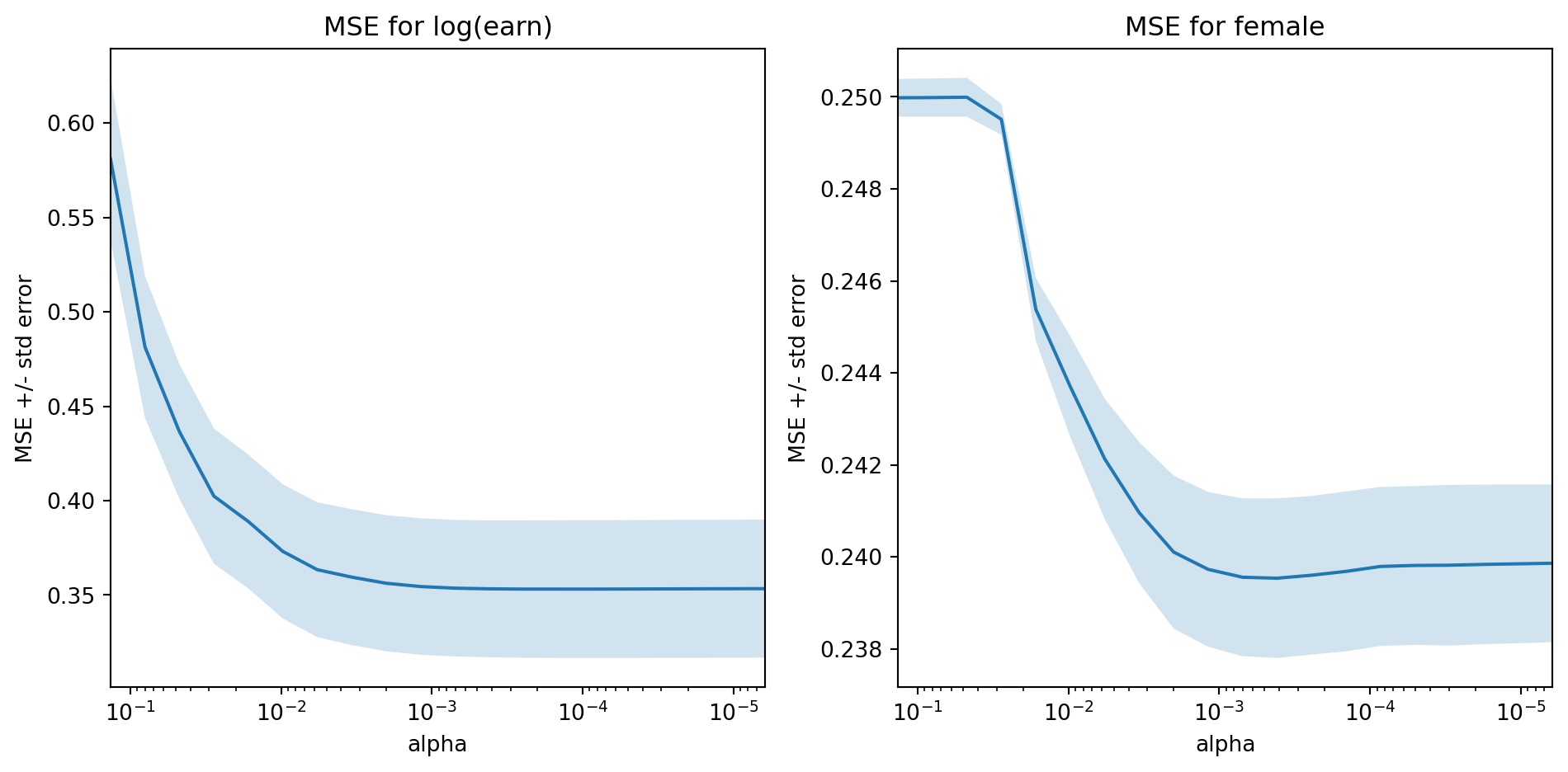
Data

import matplotlib.pyplot as plt
import numpy as np
import pandas as pd

from sklearn.model_selection import cross_val_predict
from sklearn import linear_model
from sklearn.preprocessing import PolynomialFeatures
import statsmodels as sm
import statsmodels.formula.api as smf
from statsmodels.iolib.summary2 import summary_col
import os
import requests

url = 'https://www.nber.org/morg/annual/morg23.dta'
local_filename = 'data/morg23.dta'

if not os.path.exists(local_filename):
    response = requests.get(url)
    with open(local_filename, 'wb') as file:
        file.write(response.content)

cpsall=pd.read_stata(local_filename)
# take subset of data just to reduce computation time
cps = cpsall.sample(30000, replace=False, random_state=0)
cps["female"] = (cps.sex==2)
cps["log_earn"] = np.log(cps["earnwke"])
cps["log_uhours"] = np.log(cps.uhourse)
cps["log_hourslw"] = np.log(cps.hourslw)
cps.replace(-np.inf, np.nan, inplace=True)
cps["nevermarried"] = cps.marital==7
cps["wasmarried"] = (cps.marital >= 4) & (cps.marital <= 6)
cps["married"] = cps.marital <= 3

cps.describe()

	hurespli	hhnum	county	centcity	smsastat	icntcity	smsa04	relref95	age	spouse	...	ym	ch02	ch35	ch613	ch1417	ch05	ihigrdc	log_earn	log_uhours	log_hourslw
count	29981.000000	30000.000000	30000.000000	24769.000000	29700.000000	3637.000000	30000.000000	30000.000000	30000.0000	15166.000000	...	30000.000000	30000.000000	30000.000000	30000.000000	30000.000000	30000.000000	20678.000000	15437.000000	16367.000000	16687.000000
mean	1.250325	1.039333	25.706267	1.940813	1.190067	1.407479	3.663267	42.799233	49.4125	1.587037	...	752.582333	0.054800	0.058133	0.127433	0.082300	0.093467	12.474732	6.867861	3.595133	3.566121
std	0.623380	0.208777	61.805660	0.715204	0.392361	0.954135	2.592586	3.839065	19.1787	0.702528	...	6.883342	0.227593	0.233999	0.333463	0.274826	0.291090	2.434483	0.820460	0.394975	0.488110
min	0.000000	1.000000	0.000000	1.000000	1.000000	1.000000	0.000000	40.000000	16.0000	1.000000	...	741.000000	0.000000	0.000000	0.000000	0.000000	0.000000	0.000000	-3.506558	0.000000	0.000000
25%	1.000000	1.000000	0.000000	1.000000	1.000000	1.000000	0.000000	40.000000	33.0000	1.000000	...	747.000000	0.000000	0.000000	0.000000	0.000000	0.000000	12.000000	6.461468	3.688879	3.555348
50%	1.000000	1.000000	0.000000	2.000000	1.000000	1.000000	4.000000	41.000000	50.0000	2.000000	...	753.000000	0.000000	0.000000	0.000000	0.000000	0.000000	12.000000	6.907755	3.688879	3.688879
75%	1.000000	1.000000	27.000000	2.000000	1.000000	1.000000	6.000000	42.000000	65.0000	2.000000	...	759.000000	0.000000	0.000000	0.000000	0.000000	0.000000	14.000000	7.387090	3.688879	3.688879
max	10.000000	4.000000	810.000000	3.000000	2.000000	7.000000	7.000000	59.000000	85.0000	15.000000	...	764.000000	1.000000	1.000000	1.000000	1.000000	1.000000	18.000000	9.286597	4.595120	4.595120

8 rows × 58 columns

Partial Linear Model

def partial_linear(y, d, X, yestimator, destimator, folds=3):
    """Estimate the partially linear model y = d*C + f(x) + e

    Parameters
    ----------
    y : array_like
        vector of outcomes
    d : array_like
        vector or matrix of regressors of interest
    X : array_like
        matrix of controls
    mlestimate : Estimator object for partialling out X. Must have ‘fit’
        and ‘predict’ methods.
    folds : int
        Number of folds for cross-fitting

    Returns
    -------
    ols : statsmodels regression results containing estimate of coefficient on d.
    yhat : cross-fitted predictions of y
    dhat : cross-fitted predictions of d
    """

    # we want predicted probabilities if y or d is discrete
    ymethod = "predict" if False==getattr(yestimator, "predict_proba",False) else "predict_proba"
    dmethod = "predict" if False==getattr(destimator, "predict_proba",False) else "predict_proba"
    # get the predictions
    yhat = cross_val_predict(yestimator,X,y,cv=folds,method=ymethod)
    dhat = cross_val_predict(destimator,X,d,cv=folds,method=dmethod)
    ey = np.array(y - yhat)
    ed = np.array(d - dhat)
    ols = sm.regression.linear_model.OLS(ey,ed).fit(cov_type='HC0')

    return(ols, yhat, dhat)

Unconditional Gap

lm = list()
lm.append(smf.ols(formula="log_earn ~ female", data=cps,
                  missing="drop").fit(cov_type='HC0'))
lm.append(smf.ols(formula="log_earn ~ female + log_hourslw + log_uhours", data=cps,
                  missing="drop").fit(cov_type='HC0'))
summary_col(lm, stars=True)

	log_earn I	log_earn II
Intercept	7.0101***	2.2998***
	(0.0089)	(0.0869)
female[T.True]	-0.2876***	-0.1373***
	(0.0130)	(0.0110)
log_hourslw		0.0907***
		(0.0258)
log_uhours		1.1998***
		(0.0395)
R-squared	0.0307	0.3517
R-squared Adj.	0.0307	0.3516

Standard errors in parentheses.
* p<.1, ** p<.05, ***p<.01

Adding Controls

from patsy import dmatrices
fmla  = "log_earn + female ~ log_uhours + log_hourslw + I(age**2) + age + C(grade92) + C(race) + C(smsastat) + C(unionmme) + C(unioncov) + nevermarried + wasmarried + married" #C(ind02) + C(occ2012)"
yd, X = dmatrices(fmla,cps)
female = yd[:,1]
logearn = yd[:,2];

Estimating \(\eta\)

alphas = np.exp(np.linspace(-2, -12, 20))
lassoy = linear_model.LassoCV(cv=4, alphas=alphas, max_iter=5000).fit(X,logearn)
lassod = linear_model.LassoCV(cv=4, alphas=alphas, max_iter=5000).fit(X,female);

Estimating \(\eta\)

fig, ax = plt.subplots(1,2)

def plotlassocv(l, ax) :
    alphas = l.alphas_
    mse = l.mse_path_.mean(axis=1)
    std_error = l.mse_path_.std(axis=1)
    ax.plot(alphas,mse)
    ax.fill_between(alphas, mse + std_error, mse - std_error, alpha=0.2)

    ax.set_ylabel('MSE +/- std error')
    ax.set_xlabel('alpha')
    ax.set_xlim([alphas[0], alphas[-1]])
    ax.set_xscale("log")
    return(ax)

ax[0] = plotlassocv(lassoy,ax[0])
ax[0].set_title("MSE for log(earn)")
ax[1] = plotlassocv(lassod,ax[1])
ax[1].set_title("MSE for female")
fig.tight_layout()
fig.show()

Estimating \(\eta\)

def pickalpha(lassocv) :
    #imin = np.argmin(lassocv.mse_path_.mean(axis=1))
    #msemin = lassocv.mse_path_.mean(axis=1)[imin]
    #se = lassocv.mse_path_.std(axis=1)[imin]
    #alpha= min([alpha for (alpha, mse) in zip(lassocv.alphas_, lassocv.mse_path_.mean(axis=1)) if mse<msemin+se])
    alpha = lassocv.alpha_
    return(alpha)

alphay = pickalpha(lassoy)
alphad = pickalpha(lassod)

Estimate \(\theta\)

pl_lasso = partial_linear(logearn, female, X,
                          linear_model.Lasso(alpha=alphay),
                          linear_model.Lasso(alpha=alphad))
pl_lasso[0].summary(slim=True)

OLS Regression Results

Dep. Variable:	y	F-statistic:
Model:	OLS	Prob (F-statistic):
No. Observations:	12696
Covariance Type:	HC0

	coef	std err	z	P>|z|	[0.025	0.975]
x1	-0.1856	0.010	-17.832	0.000	-0.206	-0.165

Notes:
[1] R² is computed without centering (uncentered) since the model does not contain a constant.
[2] Standard Errors are heteroscedasticity robust (HC0)

Examining Predictions

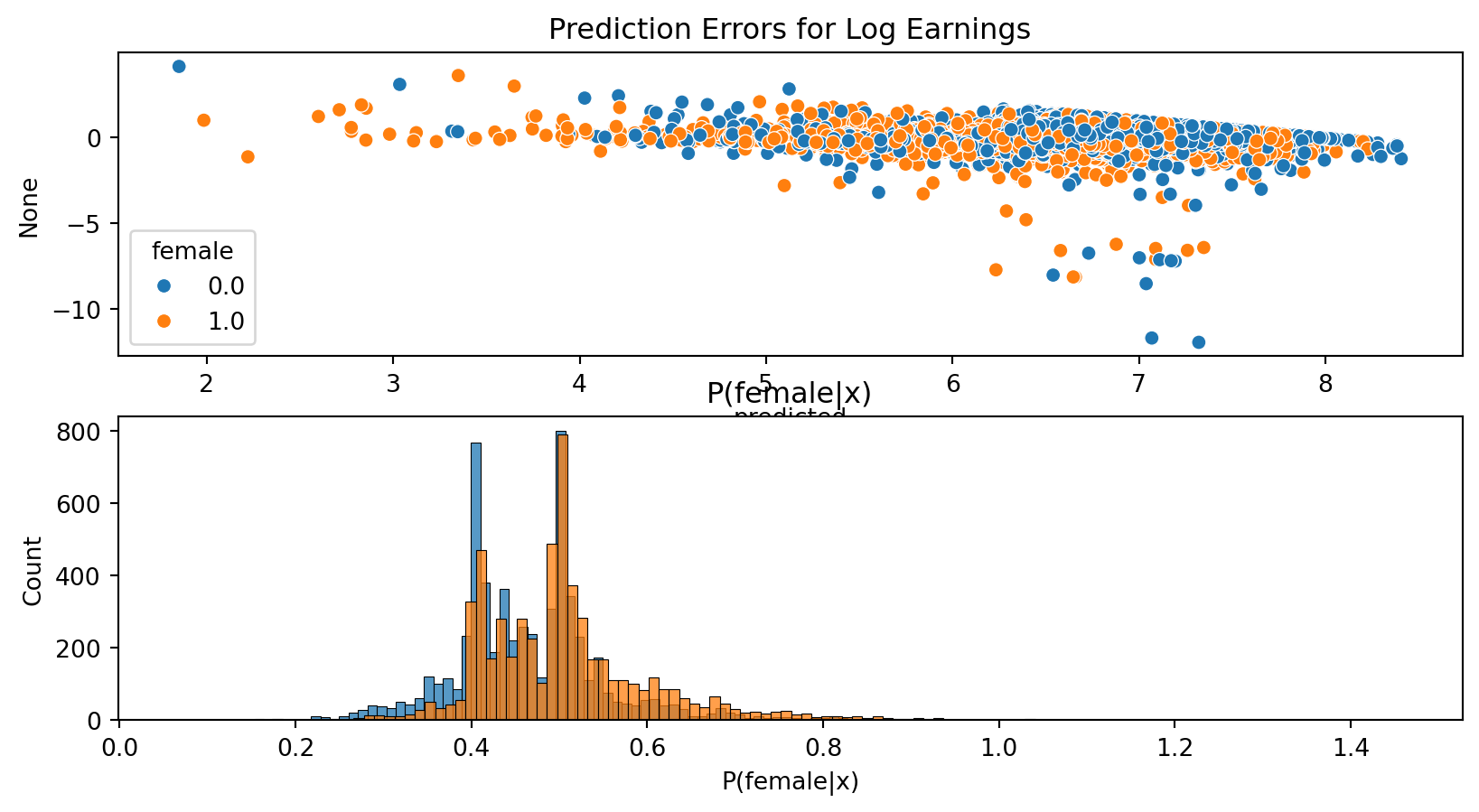
import seaborn as sns
# Visualize predictions
def preddf(pl):
    df = pd.DataFrame({"logearn":logearn,
                       "predicted":pl[1],
                       "female":female,
                       "P(female|x)":pl[2]})
    return(df)

def plotpredictions(df) :
    fig, ax = plt.subplots(2,1)
    plt.figure()
    sns.scatterplot(x = df.predicted, y = df.logearn-df.predicted, hue=df.female, ax=ax[0])
    ax[0].set_title("Prediction Errors for Log Earnings")

    sns.histplot(df["P(female|x)"][df.female==0], kde = False,
                 label = "Male", ax=ax[1])
    sns.histplot(df["P(female|x)"][df.female==1], kde = False,
                 label = "Female", ax=ax[1])
    ax[1].set_title('P(female|x)')
    return(fig)

fig=plotpredictions(preddf(pl_lasso))
fig.show()

<Figure size 960x480 with 0 Axes>

Software

• doubleml
• econml

Using doubleml

import doubleml
from sklearn.preprocessing import PolynomialFeatures
from sklearn.linear_model import LassoCV, LogisticRegressionCV
from sklearn.preprocessing import StandardScaler
from sklearn.pipeline import make_pipeline

dml_data = doubleml.DoubleMLData.from_arrays(X,logearn,female)
# Initialize learners
Cs = 0.0001*np.logspace(0, 4, 10)
lasso = make_pipeline(StandardScaler(), LassoCV(cv=5, max_iter=10000))
lasso_class = make_pipeline(StandardScaler(),
                            LogisticRegressionCV(cv=5, penalty='l1', solver='liblinear',
                                                 Cs = Cs, max_iter=1000))

np.random.seed(123)
dml_plr_lasso = doubleml.DoubleMLPLR(dml_data,
                                     ml_l = lasso,
                                     ml_m = lasso_class,
                                     n_folds = 3)
dml_plr_lasso.fit(store_predictions=True)
print(dml_plr_lasso.summary)

       coef   std err          t         P>|t|     2.5 %    97.5 %
d -0.184128  0.010433 -17.647772  1.058513e-69 -0.204577 -0.163678

Visualizing Predictions: Lasso & Logistic Lasso

def dmlpreddf(dml_model):
    df=pd.DataFrame({"logearn":logearn,
                     "predicted":dml_model.predictions['ml_l'].flatten(),
                     "female":female,
                     "P(female|x)":dml_model.predictions['ml_m'].flatten()})
    return(df)

plotpredictions(dmlpreddf(dml_plr_lasso)).show()

<Figure size 960x480 with 0 Axes>

With Gradient Boosted Trees

from lightgbm import LGBMClassifier, LGBMRegressor
ylearner = LGBMRegressor(force_col_wise=True)
dlearner = LGBMClassifier(force_col_wise=True)
dml_plr_gbt = doubleml.DoubleMLPLR(dml_data, ylearner, dlearner)
dml_plr_gbt.fit(store_predictions=True)
print(dml_plr_gbt.summary)

[LightGBM] [Info] Total Bins 299
[LightGBM] [Info] Number of data points in the train set: 10156, number of used features: 31
[LightGBM] [Info] Start training from score 6.875225
[LightGBM] [Info] Total Bins 298
[LightGBM] [Info] Number of data points in the train set: 10157, number of used features: 31
[LightGBM] [Info] Start training from score 6.867727
[LightGBM] [Info] Total Bins 296
[LightGBM] [Info] Number of data points in the train set: 10157, number of used features: 31
[LightGBM] [Info] Start training from score 6.871366
[LightGBM] [Info] Total Bins 295
[LightGBM] [Info] Number of data points in the train set: 10157, number of used features: 31
[LightGBM] [Info] Start training from score 6.873900

[LightGBM] [Info] Total Bins 294
[LightGBM] [Info] Number of data points in the train set: 10157, number of used features: 30
[LightGBM] [Info] Start training from score 6.866147
[LightGBM] [Info] Number of positive: 5021, number of negative: 5135
[LightGBM] [Info] Total Bins 299
[LightGBM] [Info] Number of data points in the train set: 10156, number of used features: 31
[LightGBM] [Info] [binary:BoostFromScore]: pavg=0.494388 -> initscore=-0.022451
[LightGBM] [Info] Start training from score -0.022451
[LightGBM] [Info] Number of positive: 5004, number of negative: 5153
[LightGBM] [Info] Total Bins 298
[LightGBM] [Info] Number of data points in the train set: 10157, number of used features: 31
[LightGBM] [Info] [binary:BoostFromScore]: pavg=0.492665 -> initscore=-0.029341
[LightGBM] [Info] Start training from score -0.029341
[LightGBM] [Info] Number of positive: 5011, number of negative: 5146
[LightGBM] [Info] Total Bins 296
[LightGBM] [Info] Number of data points in the train set: 10157, number of used features: 31
[LightGBM] [Info] [binary:BoostFromScore]: pavg=0.493354 -> initscore=-0.026584
[LightGBM] [Info] Start training from score -0.026584
[LightGBM] [Info] Number of positive: 5033, number of negative: 5124
[LightGBM] [Info] Total Bins 295
[LightGBM] [Info] Number of data points in the train set: 10157, number of used features: 31
[LightGBM] [Info] [binary:BoostFromScore]: pavg=0.495520 -> initscore=-0.017919
[LightGBM] [Info] Start training from score -0.017919
[LightGBM] [Info] Number of positive: 5003, number of negative: 5154
[LightGBM] [Info] Total Bins 294
[LightGBM] [Info] Number of data points in the train set: 10157, number of used features: 30
[LightGBM] [Info] [binary:BoostFromScore]: pavg=0.492567 -> initscore=-0.029735
[LightGBM] [Info] Start training from score -0.029735
       coef   std err          t         P>|t|     2.5 %    97.5 %
d -0.166006  0.010406 -15.952984  2.716020e-57 -0.186401 -0.145611

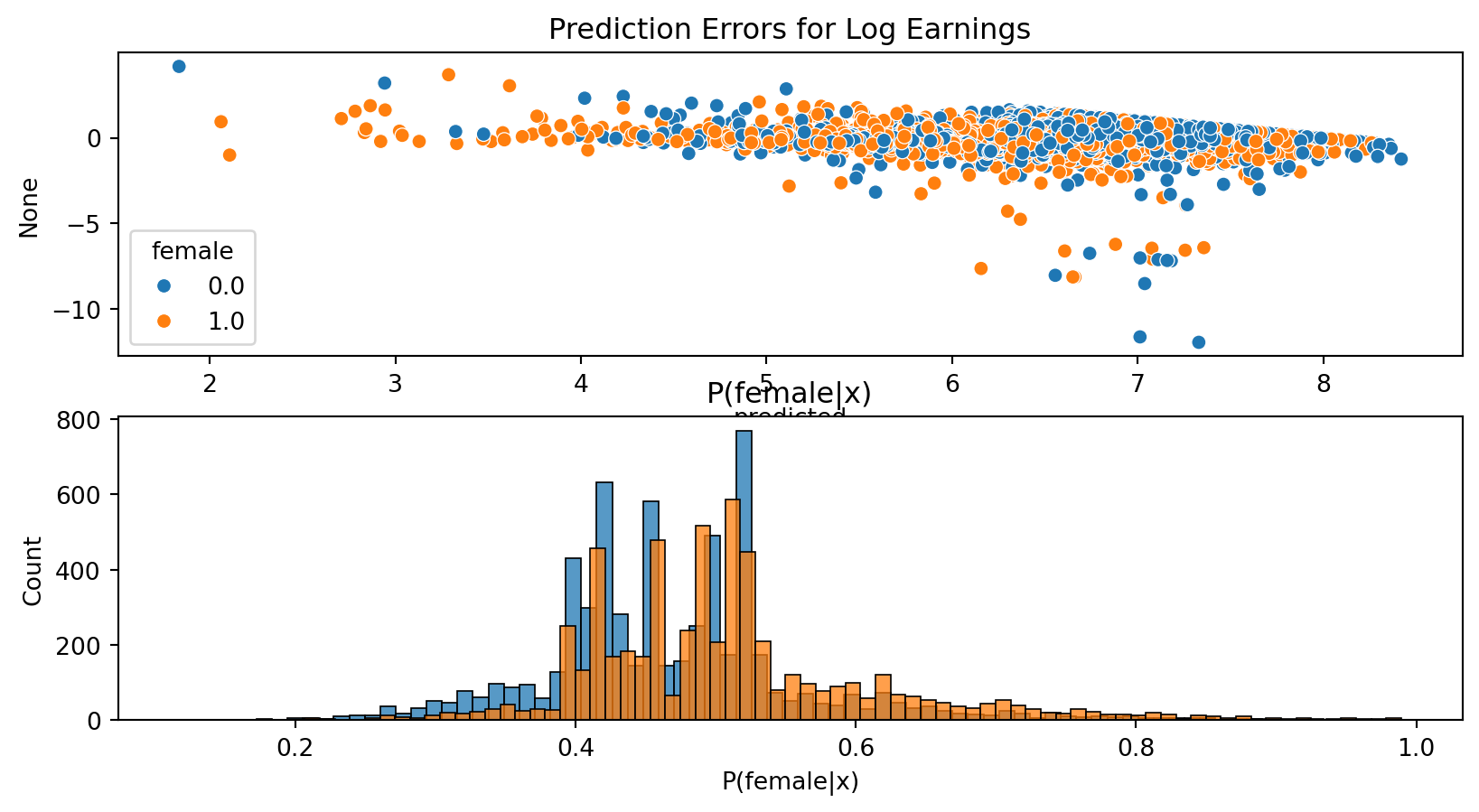
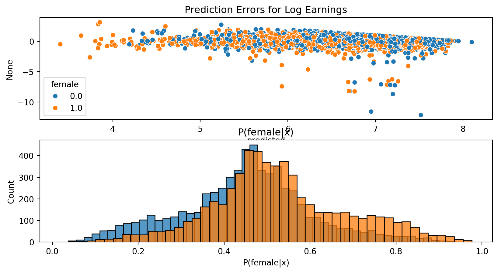
Visualizing Predictions: Trees

plotpredictions(dmlpreddf(dml_plr_gbt)).show()

<Figure size 960x480 with 0 Axes>

Interactive Regression Model

• Similar to matching, the partially linear regression model can suffer from misspecification bias if the effect of \(D\) varies with \(X\)
• Interactive regression model: \[ \begin{align*} Y & = g_0(D,X) + U \\ D & = m_0(X) + V \end{align*} \]
• Mechanics same as matching heterogeneous effects
• Orthogonal moment condition is same as doubly robust matching

Interactive Regression Model - Lasso

np.random.seed(123)
dml_irm_lasso = doubleml.DoubleMLIRM(dml_data,
                                     ml_g = lasso,
                                     ml_m = lasso_class,
                                     trimming_threshold = 0.01,
                                     n_folds = 3)
dml_irm_lasso.fit()
dml_irm_lasso.summary

	coef	std err	t	P>|t|	2.5 %	97.5 %
d	-0.192421	0.011218	-17.152773	5.992364e-66	-0.214408	-0.170434

IRM Lasso: Results

dml_irm_lasso.summary

	coef	std err	t	P>|t|	2.5 %	97.5 %
d	-0.192421	0.011218	-17.152773	5.992364e-66	-0.214408	-0.170434

dml_irm_lasso.gate(groups=pd.DataFrame(X[:,X.design_info.slice('married')])).summary

	coef	std err	t	P>|t|	[0.025	0.975]
0	-0.240815	0.015467	-15.569281	1.177236e-54	-0.27113	-0.210499

dml_irm_lasso.gate(groups=pd.DataFrame(X[:,X.design_info.slice('nevermarried')])).summary

	coef	std err	t	P>|t|	[0.025	0.975]
0	-0.118698	0.018414	-6.44594	1.148862e-10	-0.154789	-0.082606

Interactive Regression Model - Trees

np.random.seed(123)
dml_irm_gbt = doubleml.DoubleMLIRM(dml_data,
                                     ml_g = ylearner,
                                     ml_m = dlearner,
                                     trimming_threshold = 0.01,
                                     n_folds = 3)
dml_irm_gbt.fit()

[LightGBM] [Info] Total Bins 257
[LightGBM] [Info] Number of data points in the train set: 4285, number of used features: 27
[LightGBM] [Info] Start training from score 7.001738
[LightGBM] [Info] Total Bins 259
[LightGBM] [Info] Number of data points in the train set: 4285, number of used features: 27
[LightGBM] [Info] Start training from score 7.023577
[LightGBM] [Info] Total Bins 269
[LightGBM] [Info] Number of data points in the train set: 4286, number of used features: 28
[LightGBM] [Info] Start training from score 7.006350
[LightGBM] [Info] Total Bins 278
[LightGBM] [Info] Number of data points in the train set: 4179, number of used features: 29
[LightGBM] [Info] Start training from score 6.727922

[LightGBM] [Info] Total Bins 273
[LightGBM] [Info] Number of data points in the train set: 4179, number of used features: 30
[LightGBM] [Info] Start training from score 6.724012
[LightGBM] [Info] Total Bins 270
[LightGBM] [Info] Number of data points in the train set: 4178, number of used features: 27
[LightGBM] [Info] Start training from score 6.730945
[LightGBM] [Info] Number of positive: 4179, number of negative: 4285
[LightGBM] [Info] Total Bins 293
[LightGBM] [Info] Number of data points in the train set: 8464, number of used features: 30
[LightGBM] [Info] [binary:BoostFromScore]: pavg=0.493738 -> initscore=-0.025049
[LightGBM] [Info] Start training from score -0.025049
[LightGBM] [Info] Number of positive: 4179, number of negative: 4285
[LightGBM] [Info] Total Bins 288
[LightGBM] [Info] Number of data points in the train set: 8464, number of used features: 30
[LightGBM] [Info] [binary:BoostFromScore]: pavg=0.493738 -> initscore=-0.025049
[LightGBM] [Info] Start training from score -0.025049
[LightGBM] [Info] Number of positive: 4178, number of negative: 4286
[LightGBM] [Info] Total Bins 294
[LightGBM] [Info] Number of data points in the train set: 8464, number of used features: 30
[LightGBM] [Info] [binary:BoostFromScore]: pavg=0.493620 -> initscore=-0.025521
[LightGBM] [Info] Start training from score -0.025521

<doubleml.irm.irm.DoubleMLIRM at 0x7fe15750b110>

IRM Trees: Results

dml_irm_gbt.summary

	coef	std err	t	P>|t|	2.5 %	97.5 %
d	-0.175141	0.01364	-12.839952	9.793520e-38	-0.201876	-0.148407

dml_irm_gbt.gate(groups=pd.DataFrame(X[:,X.design_info.slice('married')])).summary

	coef	std err	t	P>|t|	[0.025	0.975]
0	-0.225949	0.01995	-11.32599	9.757034e-30	-0.265049	-0.186848

dml_irm_gbt.gate(groups=pd.DataFrame(X[:,X.design_info.slice('nevermarried')])).summary

	coef	std err	t	P>|t|	[0.025	0.975]
0	-0.104197	0.019944	-5.224521	1.746062e-07	-0.143286	-0.065108

Sources and Further Reading

• These slides borrow heavily from my notes on machine learning in economics
• The example is from my chapter on machine learning in QuantEcon: DataScience
• Chernozhukov et al. (2017) : short introduction to main idea
• Chernozhukov et al. (2018) : underlying theory
• Knaus (2022) : approachable review of DML for doubly robust matching

References

Belloni, Alexandre, Victor Chernozhukov, and Christian Hansen. 2014. “Inference on Treatment Effects After Selection Among High-Dimensional Controls†.” The Review of Economic Studies 81 (2): 608–50. https://doi.org/10.1093/restud/rdt044.

Chernozhukov, Victor, Denis Chetverikov, Mert Demirer, Esther Duflo, Christian Hansen, and Whitney Newey. 2017. “Double/Debiased/Neyman Machine Learning of Treatment Effects.” American Economic Review 107 (5): 261–65. https://doi.org/10.1257/aer.p20171038.

Chernozhukov, Victor, Denis Chetverikov, Mert Demirer, Esther Duflo, Christian Hansen, Whitney Newey, and James Robins. 2018. “Double/Debiased Machine Learning for Treatment and Structural Parameters.” The Econometrics Journal 21 (1): C1–68. https://doi.org/10.1111/ectj.12097.

Chernozhukov, Victor, Christian Hansen, and Martin Spindler. 2015. “Valid Post-Selection and Post-Regularization Inference: An Elementary, General Approach.” Annual Review of Economics 7 (1): 649–88. https://doi.org/10.1146/annurev-economics-012315-015826.

Knaus, Michael C. 2022. “Double machine learning-based programme evaluation under unconfoundedness.” The Econometrics Journal 25 (3): 602–27. https://doi.org/10.1093/ectj/utac015.

Oliver Hines, Karla Diaz-Ordaz, Oliver Dukes, and Stijn Vansteelandt. 2022. “Demystifying Statistical Learning Based on Efficient Influence Functions.” The American Statistician 76 (3): 292–304. https://doi.org/10.1080/00031305.2021.2021984.