import numpy as np
import pandas as pd
import matplotlib.pyplot as plt

from sklearn.tree import DecisionTreeRegressor, plot_tree
from sklearn.ensemble import RandomForestRegressor, GradientBoostingRegressor
from sklearn.neighbors import KNeighborsRegressor
from sklearn.preprocessing import StandardScaler
from sklearn.pipeline import make_pipeline
from sklearn.model_selection import train_test_split, cross_val_score, KFold
from sklearn.metrics import mean_squared_error

RANDOM_STATE = 42 # fix randomness so splits, folds, and forests are reproducibleTrees, Forests, and Boosting
Python
machine learning
decision trees
random forests
boosting
nonparametric
The third notebook in the Causal ML stream. We show a different way to be flexible: decision trees, which split the data into boxes and predict the local average. A single deep tree overfits, so we average many of them into a random forest, and we close with boosting. Trees and forests are flexible nonparametric predictors, and like everything in this stream so far, they do not identify causal effects.
Outline
Prerequisites
- Notebook 2 of this stream: ridge and lasso, variable selection, and the train/test/cross-validate recipe
- Comfort with
pandasand basic Python at the COMET-intermediate level - No prior knowledge of trees is assumed; regression trees, forests, and boosting are all introduced here
Learning Outcomes
By the end of this notebook you will be able to:
- Describe what a regression tree does: split the feature space into boxes and predict the average outcome in each box.
- Fit a single decision tree and read its splits off a diagram.
- Explain why a deep tree overfits, and identify
max_depthas its flexibility hyperparameter. - Choose the depth of a tree by cross-validation, reusing the recipe from Notebook 1.
- Explain bagging and fit a random forest, and say why averaging many trees lowers variance.
- Read a table of feature importances as a predictive diagnostic.
- Describe in one sentence how boosting differs from bagging.
- Explain why a random forest’s predictions and importances are not causal effects.
1. A Third way to be Flexible
So far this stream has shown flexibility in two different ways. In Notebook 1, k-nearest-neighbours was flexible because it averaged whatever points sat nearby, and the parameter \(k\) set how many. In Notebook 2, linear models were flexible because we could pour in covariates, and the penalty \(\lambda\) kept their coefficients in check.
This notebook introduces a third kind of flexibility. A decision tree does not measure distance and does not fit a line. It carves the feature space into rectangular boxes by asking a sequence of yes-or-no questions about one feature at a time, and to predict a new case it returns the average outcome of the training points that landed in the same box.
This will be very new to most of you, so we’ll build up to this, starting with a single tree that we can draw and read. Then we’ll watch it overfit, just as \(k=1\) KNN overfit in Notebook 1 and OLS overfit with too many controls in Notebook 2. Then we fix the overfitting by averaging many trees into a random forest, and we close with a brief look at boosting, a second way to combine trees. Throughout, we’re still predicting, and the causal turn comes in Notebook 4.
1.1 The data: back to the 401(k) households
We return to the 401(k) data from Notebook 1: one row per U.S. household, the net financial assets net_tfa (in thousands of dollars) as the target, and ten features of the household, including e401, whether the household is eligible for a 401(k). We re-use this data as we have a test MSE of about 2654 which we will try and beat, and we can ask the question that matters when choosing between methods: which one predicts new households best.
savings = pd.read_csv("datasets/Pension401k.csv")

features = ["age", "inc", "educ", "fsize", "marr",
            "twoearn", "db", "pira", "hown", "e401"]
target = "net_tfa"

y = savings[target].to_numpy()
X = savings[features]

X_train, X_test, y_train, y_test = train_test_split(
    X, y, test_size=0.3, random_state=RANDOM_STATE)

print("Training households:", len(X_train))
print("Test households    :", len(X_test))
Training households: 6940
Test households : 2975One thing we do not have to do this time is scale the features. A tree split is a question like “is income above 65?”, and the answer does not change if we measure income in dollars or in thousands of dollars: the ordering of the households is all that matters, not the units. This is different from Notebook 1, where KNN measured distance and so needed every feature on a common scale, and from Notebook 2, where the penalty acted on coefficient sizes. Trees are blind to scale, so there is no StandardScaler here except inside the KNN model we carry over for comparison.
baseline_mse = mean_squared_error(y_test, np.full_like(y_test, y_train.mean()))

knn = make_pipeline(StandardScaler(), KNeighborsRegressor(n_neighbors=15))
knn.fit(X_train, y_train)
knn_mse = mean_squared_error(y_test, knn.predict(X_test))

print(f"Predict-the-mean test MSE        : {baseline_mse:.1f}")
print(f"KNN (k=15, from Notebook 1) test MSE: {knn_mse:.1f}")
Predict-the-mean test MSE : 3708.3
KNN (k=15, from Notebook 1) test MSE: 2654.4Predicting the average savings of every household, ignoring all ten features, gives a test MSE of about 3708. That is the floor any real model must clear. The KNN model from Notebook 1 clears it at about 2654. Those two numbers, 3708 and 2654, are what we will try and beat.
2. A single decision tree
A regression tree is built greedily, one split at a time. It looks across every feature and every possible cut point, and chooses the single split that most reduces the mean squared error of the two groups it creates. Then it repeats the search inside each group, and again inside those, and so on. The result is a set of boxes, called leaves, and the prediction for any household is just the average training value in whatever leaf the household falls into.
The clearest way to see this is to grow a shallow tree, shallow enough to draw, and read it.
tree3 = DecisionTreeRegressor(max_depth=3, random_state=RANDOM_STATE)
tree3.fit(X_train, y_train)

plt.figure(figsize=(16, 8))
plot_tree(tree3, feature_names=features, filled=True, rounded=True,
          impurity=False, fontsize=9)
plt.title("A regression tree of depth 3 (leaf value = predicted net financial assets)")
plt.show()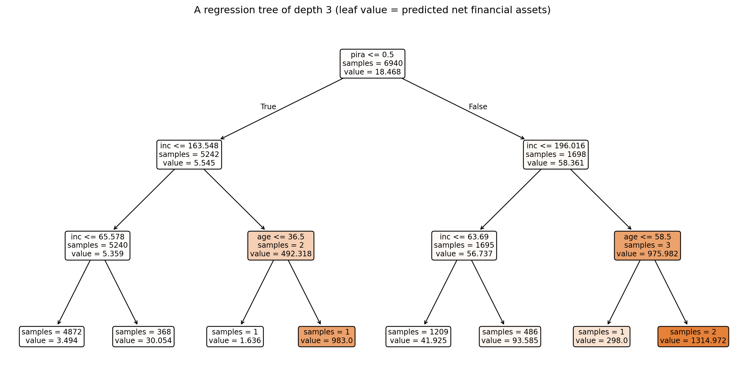
Read the tree from the top. The very first question it asks is whether the household owns an IRA (pira): owning one separates committed savers from everyone else with a single yes/no, which is why the tree chose it first. From there the splits are mostly about income, with age deciding some of the deeper ones. Follow any path down to a leaf and you reach a predicted value, and those values climb steeply: from a few thousand dollars in the leaves of low-income non-savers up into the hundreds of thousands for older, high-income IRA owners. The tree has rediscovered, with no equation, what a regression would also find: savings track income, age, and whether a household already holds retirement accounts.
print(f"Depth-3 tree test MSE: {mean_squared_error(y_test, tree3.predict(X_test)):.1f}")Depth-3 tree test MSE: 3034.7This little tree already beats predicting the mean, though it is still short of KNN. It is also easy to read, which is part of why trees are popular. But the depth-3 limit was ours to impose. What happens if we let the tree grow as deep as it likes?
2.1 When Trees overfit
If we remove the depth limit, the tree keeps splitting until it can’t anymore, in the limit isolating nearly one training household per leaf.
deep_tree = DecisionTreeRegressor(random_state=RANDOM_STATE)  # no depth limit
deep_tree.fit(X_train, y_train)

print(f"Deep tree depth        : {deep_tree.get_depth()}")
print(f"Deep tree training MSE : {mean_squared_error(y_train, deep_tree.predict(X_train)):.1f}")
print(f"Deep tree test MSE     : {mean_squared_error(y_test, deep_tree.predict(X_test)):.1f}")
Deep tree depth : 37
Deep tree training MSE : 0.0
Deep tree test MSE : 4739.5The tree grew 37 levels deep, and its training MSE is essentially zero. It has put almost every training household in a leaf of its own and reads the value straight back, so on the training data it is never wrong. We have seen this failure twice already: it is the \(k=1\) nearest-neighbour problem from Notebook 1 and the too-many-coefficients problem from Notebook 2, just with trees. The test MSE, 4739.5, is worse than the depth-3 tree, worse than KNN, and worse even than predicting the mean. A tree deep enough to memorise the training households carries none of that memorisation over to new ones.
So max_depth is the tree’s flexibility parameter, playing the role that \(k\) played for KNN and \(\lambda\) played for ridge and lasso. A shallow tree is rigid and high-bias, a deep tree is flexible and high-variance, and somewhere in between is a depth that predicts best.
2.2 Choosing the depth
We find that depth the same way we found \(k\) in Notebook 1: plot it and watch both errors.
depths = range(1, 21)
train_errors, test_errors = [], []
for d in depths:
    t = DecisionTreeRegressor(max_depth=d, random_state=RANDOM_STATE).fit(X_train, y_train)
    train_errors.append(mean_squared_error(y_train, t.predict(X_train)))
    test_errors.append(mean_squared_error(y_test, t.predict(X_test)))

best_depth_by_test = list(depths)[int(np.argmin(test_errors))]

plt.figure(figsize=(9, 6))
plt.plot(list(depths), train_errors, label="training MSE")
plt.plot(list(depths), test_errors, label="test MSE")
plt.axvline(best_depth_by_test, color="black", linestyle="--",
            label=f"lowest test MSE at depth = {best_depth_by_test}")
plt.xlabel("max_depth")
plt.ylabel("mean squared error")
plt.title("The bias-variance tradeoff for a tree: depth is the flexibility knob")
plt.legend()
plt.show()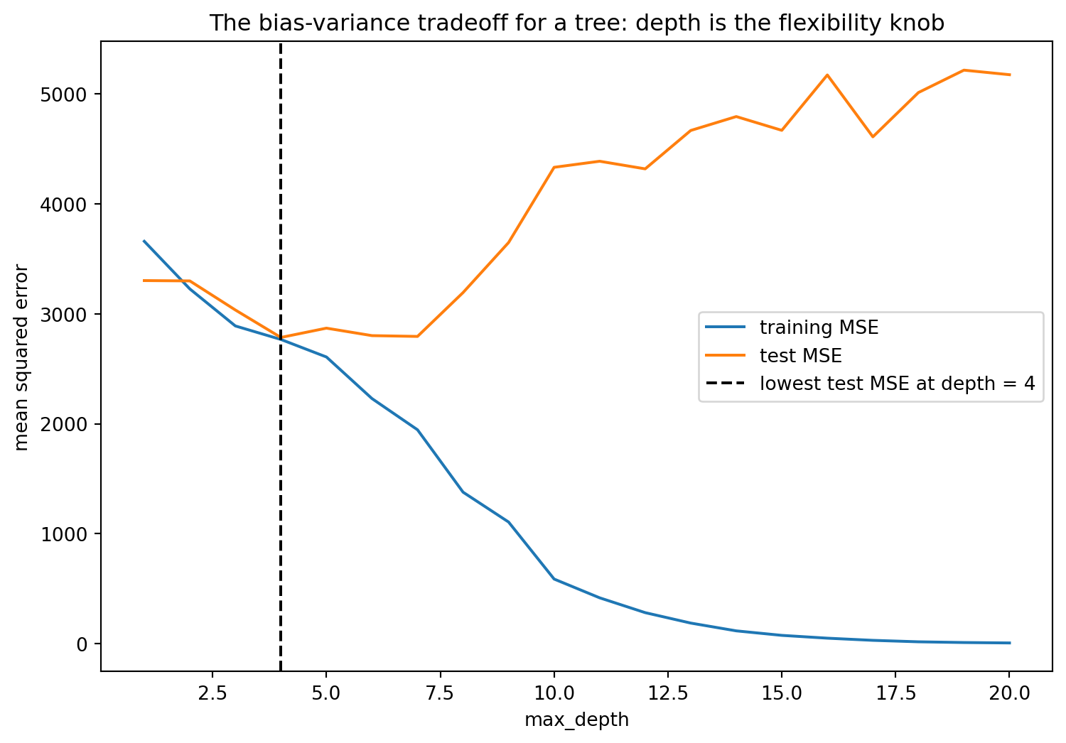
It is the same picture as Notebook 1, drawn against depth instead of \(k\), as that is the corresponding hyperparameter for trees. Training MSE falls steadily toward zero as the tree grows, because a deeper tree can always cut the training data more finely. Test MSE traces the bias-variance U-shape: shallow trees (depth 1 to 3) are too rigid and sit a little high, it bottoms out across a flat, noisy stretch from roughly depth 4 to 7, and beyond depth 8 it climbs steadily as the tree fits noise. The dashed line marks the lowest test MSE here, at depth 4, but several neighbouring depths are similar. That flat, wiggly bottom is why we don’t pick the depth by eye, and turn to cross-validation instead.
We choose it with cross-validation, never touching the test set, like in notebook 1.
kfold = KFold(n_splits=5, shuffle=True, random_state=RANDOM_STATE)

cv_errors = []
for d in depths:
    scores = cross_val_score(
        DecisionTreeRegressor(max_depth=d, random_state=RANDOM_STATE),
        X_train, y_train, cv=kfold, scoring="neg_mean_squared_error")
    cv_errors.append(-scores.mean())

best_depth = list(depths)[int(np.argmin(cv_errors))]
tree_best = DecisionTreeRegressor(max_depth=best_depth, random_state=RANDOM_STATE).fit(X_train, y_train)
tree_mse = mean_squared_error(y_test, tree_best.predict(X_test))

print(f"Cross-validation chose max_depth = {best_depth}")
print(f"Tuned single-tree test MSE: {tree_mse:.1f}")
Cross-validation chose max_depth = 4
Tuned single-tree test MSE: 2784.9Cross-validation decides on a shallow depth of 4, and the tuned tree scores just behind KNN, close enough that a single well-chosen tree is already a competitive predictor. We have now run the same four steps as in Notebook 1: split off a test set, cross-validate on the training data to choose the parameter, pick the best value, and evaluate once on the sealed test set.
The issue is that even the best single tree is a high-variance object. Shift a few training households and the greedy search can pick a different first split, and the whole tree below it rearranges. We can see that instability directly. Below we pick five test households spanning low to high savings, and ask forty trees, each fit to a different bootstrap resample of the training data, to predict each one. Bootstrapping: drawing, with replacement, many resamples of the training data the same size as the original (you may have seen this concept in ECON 226 and 326). Every grey dot is one tree’s guess; the red mark is the forest’s single answer.
forest_demo = RandomForestRegressor(n_estimators=300, random_state=RANDOM_STATE, n_jobs=-1)
forest_demo.fit(X_train, y_train)

# Five test households spanning low to high predicted savings.
order = np.argsort(forest_demo.predict(X_test))
picks = [order[int(q * (len(order) - 1))] for q in [0.2, 0.4, 0.6, 0.8, 0.9]]
X_pick = X_test.iloc[picks]

# Ask forty single trees, each fit to its own bootstrap resample, about each household.
rng = np.random.default_rng(0)
tree_guesses = np.array([
    DecisionTreeRegressor(random_state=RANDOM_STATE).fit(X_train.iloc[idx], y_train[idx]).predict(X_pick)
    for idx in (rng.integers(0, len(X_train), len(X_train)) for _ in range(40))
])

plt.figure(figsize=(9, 6))
for j in range(len(picks)):
    xj = (j + 1) + rng.uniform(-0.18, 0.18, len(tree_guesses))
    plt.scatter(xj, tree_guesses[:, j], s=14, alpha=0.4, color="grey",
                label="single trees (one dot per tree)" if j == 0 else None)
plt.scatter(range(1, len(picks) + 1), forest_demo.predict(X_pick), color="tab:red",
            s=160, marker="_", linewidth=3, zorder=5, label="random forest")
plt.xticks(range(1, len(picks) + 1), [f"household {i+1}" for i in range(len(picks))])
plt.ylim(-40, 180)
plt.ylabel("predicted net financial assets ($1,000s)")
plt.title("Ask 40 single trees about one household and they scatter; the forest gives one steady answer")
plt.legend()
plt.show()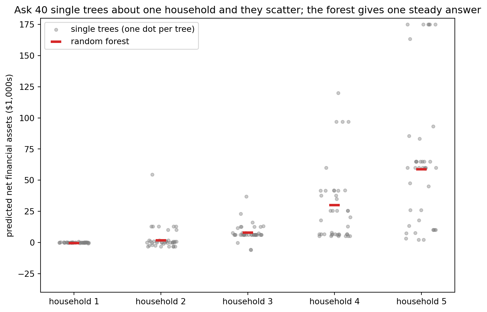
For any one household the grey dots are spread all over: ask a different resample and a single tree shifts its answer by tens of thousands of dollars. The red mark is the forest, the average of trees just like these, and it sits as one steady prediction in the middle of the scatter. The spread grows for the higher-saving households on the right, where a few extreme outcomes make any singular tree have extremely high variance.
3. Many Trees: Random Forest
A single deep tree has low bias and high variance: it captures fine structure, but its predictions can swing a lot when the training data changes, just as the grey dots above showed. We fix this by taking the average. If we had many trees, each fit to a slightly different sample, their individual errors would partly cancel when we averaged their predictions, while the structure they agree on would survive.
We do not have many samples, but we can manufacture them by bootstrapping. We fit a deep tree to each resample and average their predictions. This is called bagging, short for bootstrap aggregating, and it keeps the low bias of deep trees while cutting their variance.
A random forest adds one more idea. At each split, each tree is allowed to consider only a random handful of the features, not all ten. This stops every tree from opening with the same IRA split and makes the trees less alike, so their errors cancel more thoroughly when averaged. It leads to a bit more bias per tree, but we get a significant drop in variance instead.
forest = RandomForestRegressor(n_estimators=300, random_state=RANDOM_STATE, n_jobs=-1)
forest.fit(X_train, y_train)

forest_mse = mean_squared_error(y_test, forest.predict(X_test))
print(f"Random forest training MSE: {mean_squared_error(y_train, forest.predict(X_train)):.1f}")
print(f"Random forest test MSE    : {forest_mse:.1f}")
Random forest training MSE: 473.8
Random forest test MSE : 2837.7The forest scores 2837.7 on the test set. Notice the training MSE: it is far from zero, even though each individual tree in the forest still memorises its own bootstrap sample. Averaging across 300 trees pulls the aggregate away from memorisation, and that’s why the forest generalizes well, when a single deep tree did not. On this data the forest is similar to a tuned-tree and KNN.
3.1 Feature Importance
A forest cannot be drawn as one readable diagram, but it can tell us how much each feature contributed to reducing MSE across all the splits in all the trees. This is called feature importance.
importances = pd.Series(forest.feature_importances_, index=features).sort_values()

plt.figure(figsize=(9, 6))
plt.barh(importances.index, importances.values)
plt.xlabel("importance (share of total MSE reduction)")
plt.title("Random forest feature importances")
plt.show()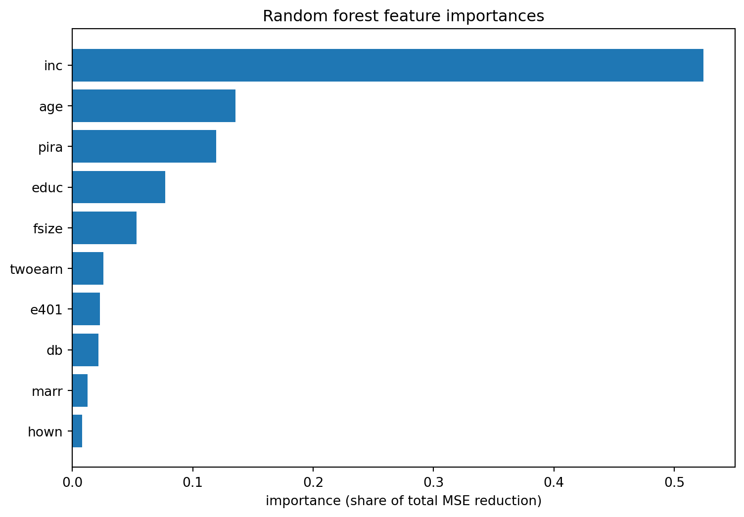
Income is by far the most useful feature, followed by age and owning an IRA. This matches what we read off the single tree. Look at e401 in that graph, the eligibility for a 401(k) variable that this whole stream is building toward. It is near the very bottom, barely used by the forest at all. It’s a useful diagnostic, but a predictive one. We will find out in notebook 8 that its predictive power says nothing about its true effect.
4. Boosting
Bagging and forests build many trees in parallel and average them. Boosting builds trees in sequence. The first tree makes its predictions, and the next tree is fit not to the outcome but to the errors the first one left behind, so it spends its effort on the cases the aggregate is getting wrong. Add a third tree fit to what the first two still miss, repeated over many rounds. The trees are kept deliberately shallow, because each one only has to nudge the running prediction a little.
We can watch the running prediction build up. Below we boost on income alone so we can draw it, and plot the ensemble’s fit after 1 round, after 10, and after 100.
inc1 = X_train[["inc"]]
inc_grid = pd.DataFrame({"inc": np.linspace(inc1["inc"].min(), inc1["inc"].max(), 200)})

gb = GradientBoostingRegressor(n_estimators=200, max_depth=2, random_state=RANDOM_STATE)
gb.fit(inc1, y_train)
stage_preds = list(gb.staged_predict(inc_grid))

plt.figure(figsize=(9, 6))
plt.scatter(inc1["inc"], y_train, s=8, alpha=0.1, color="grey")
for n in [1, 10, 100]:
    plt.plot(inc_grid["inc"], stage_preds[n - 1], linewidth=2, label=f"{n} round(s)")
plt.ylim(-10, 120)
plt.xlabel("income ($1,000s)")
plt.ylabel("predicted net financial assets ($1,000s)")
plt.title("Boosting builds up: each round fits the errors the last ones left")
plt.legend()
plt.show()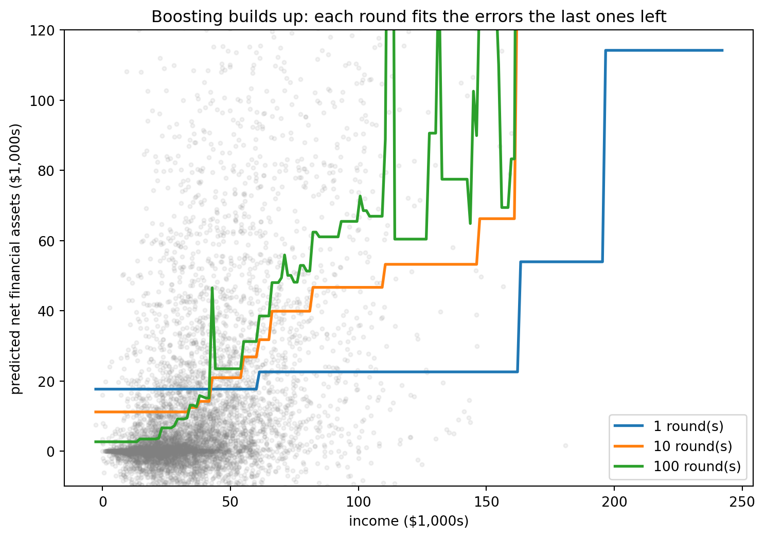
After one round the fit is a simple step function. After ten it has bent toward the data. After one hundred it traces the income-savings relationship even closer, having spent each new tree on whatever the running total still got wrong. Now we fit the full boosted model on all ten features.
boosted = GradientBoostingRegressor(random_state=RANDOM_STATE)
boosted.fit(X_train, y_train)
boosted_mse = mean_squared_error(y_test, boosted.predict(X_test))

print(f"Gradient boosting test MSE: {boosted_mse:.1f}")
Gradient boosting test MSE: 2593.4Out of the box, boosting is the best predictor we have built on this data, ahead of KNN and the forest. The gap is small, and it can be improved further with some fine tuning; the point for us is not which tree ensemble wins by a few percent, but that both bagging and boosting take the overfitting tree from section 2 and turn it into a powerful predictor. In practice the boosting idea is taken further by libraries like XGBoost and LightGBM, which are among the most reliable predictors in everyday use, but the mechanism is the one we just learned about.
We stop at tree ensembles. Neural networks are another flexible predictor, you can read more about them in this notebook.
5. So have we found the effect of 401(k) eligibility?
Let us line up every model we have fit on this same split.
results = pd.DataFrame({
    "model": ["Predict the mean", "KNN (k=15)", "Single tree (tuned)",
              "Random forest", "Gradient boosting"],
    "test MSE": [baseline_mse, knn_mse, tree_mse, forest_mse, boosted_mse],
})
print(results.round(1).to_string(index=False))
model test MSE
Predict the mean 3708.3
KNN (k=15) 2654.4
Single tree (tuned) 2784.9
Random forest 2837.7
Gradient boosting 2593.4The flexible methods all beat the baseline and land close together, with boosting a bit ahead of the others. So we now have a decent predictor of household savings. Time for the question this stream keeps returning to:
Do any of these models tell us the effect of 401(k) eligibility on a household’s savings?
No! Look back at the model comparison: the flexible methods cluster together, and they got there by chasing whatever predicts savings. The tree opened on owning an IRA because that variable splits savers from everyone else with the most predictive power, not because we ever showed that owning an IRA causes savings, and the forest utilizes income and age for the same reason. Meanwhile e401, the eligibility variable this whole stream is building toward, sat near the bottom of the importance plot, almost useless for prediction because eligible and ineligible households already look so different. But that low importance says nothing about its effect: Notebook 4 builds a world where eligibility has a real, positive effect that a naive comparison still gets wrong, and the public-economics literature finds a real effect too. And no forest (or other predictive technique), ever imagines this household made eligible with everything else held fixed, which is the counterfactual a causal answer requires. A model can be a fine predictor and still be useless for the effect we came here to measure. Notebook 4 makes the turn and explains what identifying a treatment effect actually requires.
Its causal future
The random forest comes back later in a causal disguise. Notebook 8’s causal forest reuses this notebook’s ideas, re-aimed from predicting an outcome to estimating how a treatment effect varies from one household to the next.
Connections
- Back to Notebook 2: ridge and lasso were flexible linear models, controlled by a penalty.
- Forward to Notebook 4: we now have learned three prediction tools and still cannot answer a causal question with any of them. Notebook 4 explains why, and what identification requires that prediction does not, and why.
References
- Breiman, L. (1996). Bagging predictors. Machine Learning, 24(2), 123-140.
- Breiman, L. (2001). Random forests. Machine Learning, 45(1), 5-32.
- Chernozhukov, V., Hansen, C., & Spindler, M. (2016). hdm: High-dimensional metrics. R Journal, 8(2), 185-199. The source of the 401(k) dataset.
- Friedman, J. H. (2001). Greedy function approximation: a gradient boosting machine. Annals of Statistics, 29(5), 1189-1232.
- GeeksforGeeks. (2025). Feature importance with random forests. GeeksforGeeks. https://www.geeksforgeeks.org/machine-learning/feature-importance-with-random-forests/
- James, G., Witten, D., Hastie, T., & Tibshirani, R. (2021). An Introduction to Statistical Learning. Springer. (Chapter 8.)
- scikit-learn developers. (n.d.). 1.10. Decision trees. scikit-learn. https://scikit-learn.org/stable/modules/tree.html
- Wikipedia contributors. (2025). Bootstrap aggregating. Wikipedia. https://en.wikipedia.org/wiki/Bootstrap_aggregating
- Wikipedia contributors. (n.d.). Random forest. Wikipedia. https://en.wikipedia.org/wiki/Random_forest