import numpy as np
import pandas as pd
import matplotlib.pyplot as plt

from sklearn.linear_model import LinearRegression, Ridge, Lasso, RidgeCV, LassoCV
from sklearn.preprocessing import StandardScaler
from sklearn.pipeline import make_pipeline
from sklearn.model_selection import train_test_split
from sklearn.metrics import mean_squared_error, r2_score

RANDOM_STATE = 42 # fix randomness so splits and folds are reproducibleRegularization: Ridge and Lasso
Python
machine learning
regularization
ridge
lasso
variable selection
The second notebook in the Causal ML stream. We encounter the ‘too many controls’ problem, where ordinary least squares falls apart once the number of covariates approaches the number of observations, and we fix it with regularization: ridge and lasso, the coefficient path, and the idea that lasso selects variables.
Outline
Prerequisites
- Notebook 1 of this stream: train/test splits, MSE, the bias-variance tradeoff, k-fold cross-validation, and the Machine Learning
Pipeline - Multiple regression and OLS (COMET Intermediate: Introduction to Regression, Multiple Regression)
- Comfort with
pandasand basic Python at the COMET-intermediate level
Learning Outcomes
By the end of this notebook you will be able to:
- Explain why OLS falls apart when the number of covariates approaches or exceeds the number of observations.
- State what regularization does: trade a little bias for a large drop in variance.
- Fit a ridge regression and explain the role of the penalty \(\lambda\).
- Read a coefficient path and describe how the coefficients shrink as \(\lambda\) grows.
- Fit a lasso regression and articulate why lasso = variable selection.
- Say when you would use ridge versus lasso.
- Choose \(\lambda\) by cross-validation, reusing the method learned in Notebook 1.
- Explain why a lasso-selected coefficient is not yet a causal effect.
1. The “Too Many Controls” Problem
In Notebook 1 we learned that flexibility is a double-edged sword: the more freedom we give a model, the better it fits the data in front of it and the worse it can do on data it has not seen. KNN made that easy to see by setting one hyperparameter, \(k\). This notebook continues with this concept using a technique you have already learned, ordinary least squares.
OLS has a hyperparameter we can set too, though we rarely think of it that way: the number of regressors. Each control we add gives the model one more degree of freedom to bend toward the data. Add enough of them and the model can fit the training sample perfectly while learning that carries over for data it has not seen. The extreme case is when we have almost as many controls as observations, which is what happens when you want to “control for everything.”
This notebook has a concrete question behind it. One of the oldest debates in growth economics is convergence: do countries that start poor grow faster and catch up to the rich ones? Answering it means measuring the effect of a country’s initial wealth on its later growth while holding fixed everything else that shapes growth, its schooling, its institutions, its openness to trade, etc. This question is an example of wishing to “control for everything”, where the convergence coefficient is what we’re after and dozens of possible controls stand between us and a clean reading of it.
The question for this notebook is what to do when that happens. We’ll watch OLS fail on a real dataset, and then meet two ways to rescue it, ridge and lasso, which both work by stopping the coefficients from growing without limit.
1.1 The Growth Data
We will use the Barro-Lee growth data, a standard dataset in the study of economic growth. Each row is a country. The outcome is Outcome, the country’s average annual growth rate of GDP per capita over the period. The variable gdpsh465 is the log of GDP per capita at the start of the period (1965), and the remaining columns are country characteristics measured around the same time: schooling and education rates, government spending, trade and market openness, political stability, and various other demographics. These variables have special codes: 65 means the variable was measured in 1965, a trailing m or f marks male or female, and a schooling prefix marks the level, p for primary, s for secondary, h or high for higher, no for none. human is an average-years-of-schooling measure. So pf65 is female primary schooling in 1965, highm65 is male higher schooling, and humanm65 is average male schooling.
We will load the data:
growth = pd.read_csv("datasets/GrowthData.csv")

target = "Outcome"
y = growth[target].to_numpy()
X = growth.drop(columns=[target])

print("Countries (observations):", X.shape[0])
print("Covariates:", X.shape[1])
X.iloc[:5, :6]
Countries (observations): 90
Covariates: 61| gdpsh465 | bmp1l | freeop | freetar | h65 | hm65 | |
|---|---|---|---|---|---|---|
| 0 | 6.591674 | 0.2837 | 0.153491 | 0.043888 | 0.007 | 0.013 |
| 1 | 6.829794 | 0.6141 | 0.313509 | 0.061827 | 0.019 | 0.032 |
| 2 | 8.895082 | 0.0000 | 0.204244 | 0.009186 | 0.260 | 0.325 |
| 3 | 7.565275 | 0.1997 | 0.248714 | 0.036270 | 0.061 | 0.070 |
| 4 | 7.162397 | 0.1740 | 0.299252 | 0.037367 | 0.017 | 0.027 |
So we have 90 countries and 61 covariates. 61 coefficients to fit 90 numbers leaves almost no room to spare, and once we split off a test set it gets far worse.
A note on scaling, which mattered in Notebook 1 and matters even more here. Ridge and lasso work by penalizing the size of the coefficients, and the size of a coefficient depends on the units of its variable, a coefficient on income measured in dollars is a thousand times smaller than the same effect measured in thousands of dollars. If we penalize coefficients without first putting the variables on a common scale, the penalty falls unevenly. So we standardize every feature, and as in Notebook 1 we do it inside a pipeline so that the scaling is always learned from the training data alone.
2. Why OLS breaks with many covariates
We split off a test set exactly as before, holding out 30% of the countries.
X_train, X_test, y_train, y_test = train_test_split(
    X, y, test_size=0.3, random_state=RANDOM_STATE)

print("Training countries:", len(X_train))
print("Test countries    :", len(X_test))
Training countries: 63
Test countries : 27Now there are 63 countries in the training set and 61 covariates. Counting the intercept, that is 62 free coefficients to fit 63 points, so OLS has almost no room to spare and can bend nearly all the way to the training data. Let’s see what that does.
ols = make_pipeline(StandardScaler(), LinearRegression())
ols.fit(X_train, y_train)

ols_train_mse = mean_squared_error(y_train, ols.predict(X_train))
ols_test_mse = mean_squared_error(y_test, ols.predict(X_test))
baseline_mse = mean_squared_error(y_test, np.full_like(y_test, y_train.mean()))

print(f"OLS training R^2 : {r2_score(y_train, ols.predict(X_train)):.3f}")
print(f"OLS training MSE : {ols_train_mse:.5f}")
print(f"OLS test MSE     : {ols_test_mse:.5f}")
print(f"Predict-the-mean test MSE: {baseline_mse:.5f}")
OLS training R^2 : 1.000
OLS training MSE : 0.00000
OLS test MSE : 0.03663
Predict-the-mean test MSE: 0.00340The training \(R^2\) is 1 and the training MSE is 0: OLS fits the countries it was trained on almost perfectly. But the test MSE is ten times larger than what we would get by ignoring every covariate and just predicting the average growth rate. A model with 61 controls does worse than a model with none. This is the same overfitting we saw in Notebook 1 with the \(k=1\) nearest neighbour, only in a different setting, because with so little room to spare OLS fits the noise in the training countries and carries none of it over to new ones.
This can be seen even more clearly in the coefficients OLS chose.
ols_coefs = pd.Series(ols[-1].coef_, index=X.columns)

plt.figure(figsize=(9, 6))
plt.bar(range(len(ols_coefs)), ols_coefs.values, color="tab:red")
plt.axhline(0, color="black", linewidth=0.8)
plt.xlabel("covariate (one bar each)")
plt.ylabel("OLS coefficient (standardized features)")
plt.title("OLS coefficients run wild")
plt.show()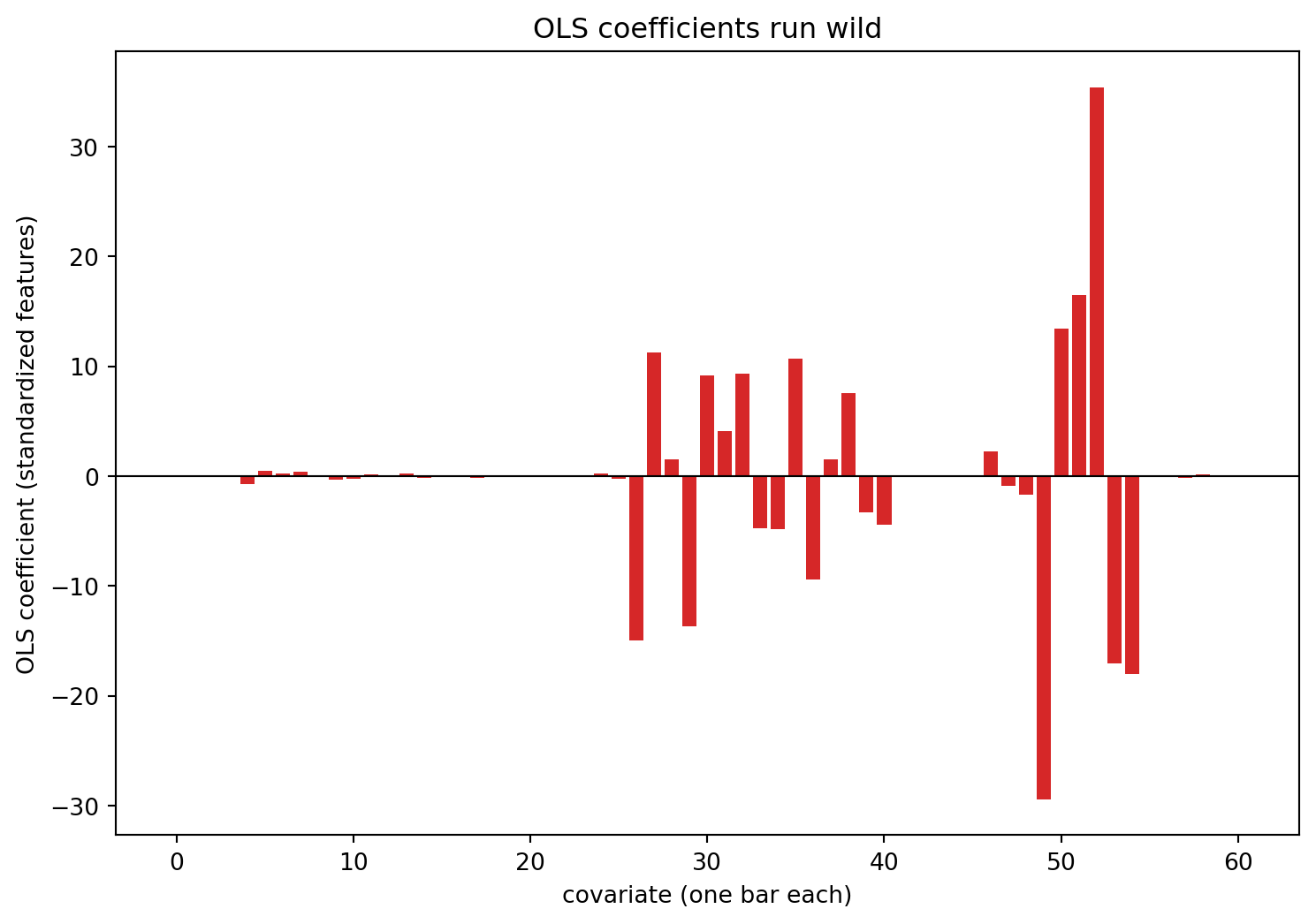
The growth outcome is a small number (an annual rate of a few percent), yet some of these coefficients reach into the tens. OLS is throwing large positive and negative weights at correlated covariates so that they nearly cancel on the training countries, which is how it drives training error to zero when it has no room to spare. Those huge offsetting weights are what fall apart on new countries. Ridge and lasso, which are coming up, are ways to stop this from happening.
We cannot drop covariates by hand without knowing which ones matter, and we do not want to throw away information. The fix is to keep all 61 covariates but stop their coefficients from running wild. This is called regularization.
3. Ridge regression
Ridge keeps the OLS goal of making the residuals small, but adds a price for large coefficients. It minimises
\[ \sum_{i=1}^{n} \left( y_i - \hat{y}_i \right)^2 \;+\; \lambda \sum_{j=1}^{p} \beta_j^2 . \]
The first term is the usual sum of squared residuals (OLS). The second is the penalty: the squared size of the coefficients, scaled by a number \(\lambda\) we choose. When \(\lambda = 0\) there is no penalty and ridge is just OLS. As \(\lambda\) grows, large coefficients become expensive, so the fit pulls them toward zero. In the limit of huge \(\lambda\) every coefficient is squeezed to nearly nothing and the model predicts close to a constant.
The clearest way to see this is the coefficient path: fit ridge at many values of \(\lambda\) and plot how each coefficient moves.
scaler = StandardScaler().fit(X_train)
X_train_s = scaler.transform(X_train)

lambdas = np.logspace(-2, 4, 60)
ridge_coefs = np.array([Ridge(alpha=l).fit(X_train_s, y_train).coef_ for l in lambdas])

# Label only the few largest coefficients so the legend stays readable.
biggest = np.argsort(np.abs(ridge_coefs[0]))[-4:]

plt.figure(figsize=(9, 6))
plt.plot(lambdas, ridge_coefs, color="lightgrey", linewidth=1)
for j in biggest:
    plt.plot(lambdas, ridge_coefs[:, j], linewidth=2, label=X.columns[j])
plt.xscale("log")
plt.axhline(0, color="black", linewidth=0.8)
plt.xlabel(r"$\lambda$ (penalty strength)")
plt.ylabel("coefficient")
plt.title("Ridge coefficient path: every coefficient shrinks toward zero")
plt.legend()
plt.show()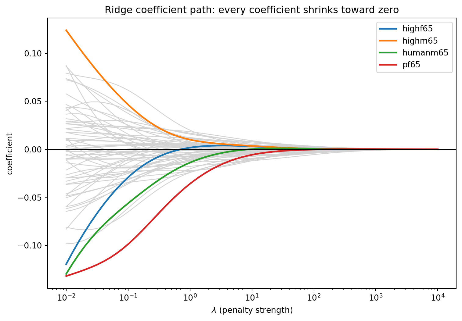
On the left, where \(\lambda\) is small, the coefficients are large and spread out: this is the unstable OLS fit from section 2. As we move right and the penalty grows, every line drifts smoothly toward zero, though nothing ever becomes exactly zero, it just keeps approaching it. The penalty is buying us stability: by refusing to let any coefficient grow large, ridge trades a little bias for a large reduction in variance. That is the same bias-variance tradeoff from Notebook 1, now showing up in a different model.
In a live session (Local or Jupyter/Colab) we can see this penalty at work. Drag \(\lambda\) below and watch the OLS coefficients on the left collapse toward zero as the penalty tightens.
from ipywidgets import interact, FloatLogSlider

def show_ridge(lam):
    c = Ridge(alpha=lam).fit(X_train_s, y_train).coef_
    plt.figure(figsize=(9, 5))
    plt.bar(range(len(c)), c, color="tab:purple")
    plt.axhline(0, color="black", linewidth=0.8)
    plt.ylim(-25, 25)
    plt.xlabel("covariate")
    plt.ylabel("coefficient")
    plt.title(f"Ridge at lambda = {lam:.2g}: largest coefficient = {np.abs(c).max():.3f}")
    plt.show()

interact(show_ridge, lam=FloatLogSlider(value=1e-6, base=10, min=-6, max=-2, step=0.2));
We still have to choose \(\lambda\). As in Notebook 1 we let cross-validation do it, which the RidgeCV function runs for us over a grid of candidates.
ridge = make_pipeline(StandardScaler(), RidgeCV(alphas=np.logspace(-2, 4, 60)))
ridge.fit(X_train, y_train)

print(f"Ridge chose lambda = {ridge[-1].alpha_:.3f}")
Ridge chose lambda = 17.957
Standardize before you penalize
A penalty on the coefficients only makes sense if the coefficients are comparable, and they are comparable only if the features share a scale. This is why the StandardScaler sits inside the pipeline: every time ridge is fit, the scaling is recomputed from just that data. Skip it and the penalty quietly punishes whichever variables happen to be measured in small units, which leads to bias that is easy to avoid.
4. Lasso
Lasso changes one thing about ridge: it penalizes the absolute size of the coefficients instead of the squared size. It minimises
\[ \sum_{i=1}^{n} \left( y_i - \hat{y}_i \right)^2 \;+\; \lambda \sum_{j=1}^{p} \left| \beta_j \right| . \]
Where ridge shrinks coefficients smoothly toward zero, lasso pushes them exactly to zero and leaves them there. A coefficient of zero means the variable is dropped from the model, so lasso doesn’t only shrink the coefficients, it also selects which ones to keep. This is the key difference between ridge and lasso.
The coefficient path makes the difference visible.
lasso_lambdas = np.logspace(-4, 0, 60)
lasso_coefs = np.array(
    [Lasso(alpha=l, max_iter=100000).fit(X_train_s, y_train).coef_ for l in lasso_lambdas])

biggest = np.argsort(np.abs(lasso_coefs[0]))[-4:]

plt.figure(figsize=(9, 6))
plt.plot(lasso_lambdas, lasso_coefs, color="lightgrey", linewidth=1)
for j in biggest:
    plt.plot(lasso_lambdas, lasso_coefs[:, j], linewidth=2, label=X.columns[j])
plt.xscale("log")
plt.axhline(0, color="black", linewidth=0.8)
plt.xlabel(r"$\lambda$ (penalty strength)")
plt.ylabel("coefficient")
plt.title("Lasso coefficient path: coefficients hit exactly zero, one by one")
plt.legend()
plt.show()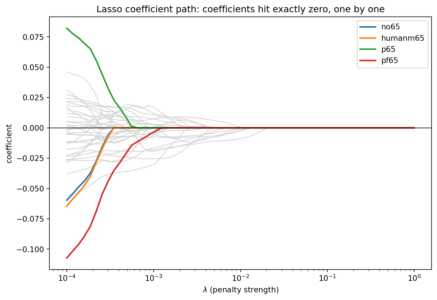
Read this plot from right to left. On the right, where the penalty is strong, every coefficient is zero: the model is empty. As we relax \(\lambda\) and move left, variables switch on one at a time, their coefficients lifting off zero. The most useful predictors enter first, and the rest stay switched off until the penalty is weak enough to afford them. At any given \(\lambda\), the model uses only the handful of variables that have entered so far.
We choose \(\lambda\) by cross-validation again, with the LassoCV function, and check how many variables aren’t zero.
lasso = make_pipeline(StandardScaler(), LassoCV(cv=5, random_state=RANDOM_STATE, max_iter=200000))
lasso.fit(X_train, y_train)

coefs = pd.Series(lasso[-1].coef_, index=X.columns)
selected = coefs[coefs != 0]

print(f"Lasso chose lambda = {lasso[-1].alpha_:.5f}")
print(f"Variables kept: {len(selected)} of {len(coefs)}")
print("\nSelected variables:")
print(selected.round(4).to_string())
Lasso chose lambda = 0.00303
Variables kept: 14 of 61
Selected variables:
gdpsh465 -0.0107
bmp1l -0.0132
hf65 -0.0105
pm65 0.0040
gpop1 -0.0077
geerec1 -0.0062
gde1 0.0011
gvxdxe41 -0.0117
pinstab1 -0.0075
worker65 0.0010
seccm65 0.0044
teasec65 0.0011
im1 0.0083
tot1 -0.0015Out of 61 covariates, lasso keeps 14 and sets the other 47 to exactly zero. It gave us a short list of the variables that carry the predictive signal, and gdpsh465, the country’s initial GDP, is on it. This is the headline of the notebook: lasso = variable selection. Ridge would have kept all 61, with each shrinking, whereas lasso keeps a few and discards the rest.
Self-test
Why does the absolute-value penalty zero coefficients out, while the squared penalty only shrinks them?
Show / hide answer
Think of the cost of moving a coefficient from a tiny value to exactly zero. Under the squared penalty the saving from that last step is itself tiny (the derivative of \(\beta^2\) vanishes at zero), so there is never quite enough reason to finish the job. Under the absolute-value penalty the saving is the same constant \(\lambda\) all the way down, including the final step to zero, so once a variable is not pulling its weight, lasso sets it to zero outright.5. Choosing between Ridge and Lasso
Both methods solve the problem from section 3, and both will beat OLS by a wide margin in the next section. They differ in variable selection.
| Ridge | Lasso | |
|---|---|---|
| Penalty | squared coefficients | absolute coefficients |
| Effect | shrinks all coefficients | shrinks and zeros some coefficients |
| Variables kept | all of them | a selected few |
| Good when | many small effects, correlated predictors | a few variables that really matter |
Ridge is the better choice when you believe most covariates contribute a little and you mainly want stability, especially when predictors are correlated and OLS cannot tell them apart. Lasso is the better choice when you believe only a few covariates matter and you want a short, interpretable model.
Putting the two fitted coefficient vectors side by side makes the difference concrete.
ridge_c = pd.Series(ridge[-1].coef_, index=X.columns)
lasso_c = pd.Series(lasso[-1].coef_, index=X.columns)
order = ridge_c.abs().sort_values().index

fig, ax = plt.subplots(1, 2, figsize=(11, 8), sharey=True)
ax[0].barh(range(len(order)), ridge_c[order].values, color="tab:blue")
ax[0].set_title("Ridge: all 61 kept, all shrunk")
ax[1].barh(range(len(order)), lasso_c[order].values, color="tab:green")
ax[1].set_title("Lasso: most are exactly zero")
for a in ax:
    a.axvline(0, color="black", linewidth=0.8)
    a.set_yticks([])
ax[0].set_ylabel("the 61 covariates")
plt.show()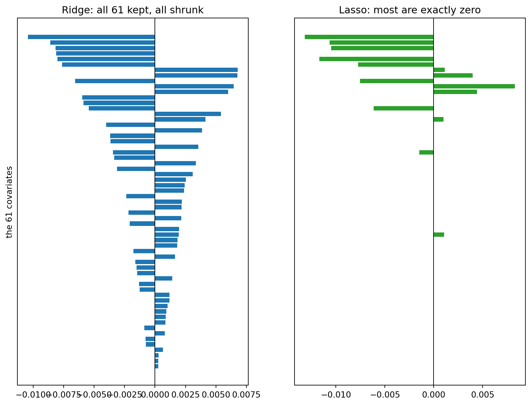
Ridge fills both columns: every covariate keeps a small nonzero weight. Lasso leaves most of its bars at exactly zero and spends real weight on only a handful, so here we can see variable selection drawn as a picture.
6. Choosing \(\lambda\) by cross-validation
We utilized RidgeCV and LassoCV above without really learning what they do, so let us make it explicit, because it is the same method as Notebook 1 showed us. To choose \(\lambda\) we never touch the test set. Instead we split the training data into folds, fit at each candidate \(\lambda\) on most of the folds, score on the held-out fold, and average. LassoCV keeps the whole grid of scores, so we can plot the cross-validation curve and see the choice it made.
lasso_cv = lasso[-1]
mean_cv_mse = lasso_cv.mse_path_.mean(axis=1)

plt.figure(figsize=(9, 6))
plt.plot(lasso_cv.alphas_, mean_cv_mse, label="5-fold CV MSE")
plt.axvline(lasso_cv.alpha_, color="black", linestyle="--",
            label=f"CV picks lambda = {lasso_cv.alpha_:.4f}")
plt.xscale("log")
plt.xlabel(r"$\lambda$ (penalty strength)")
plt.ylabel("cross-validated MSE")
plt.title("Choosing lambda with cross-validation (no peeking at the test set)")
plt.legend()
plt.show()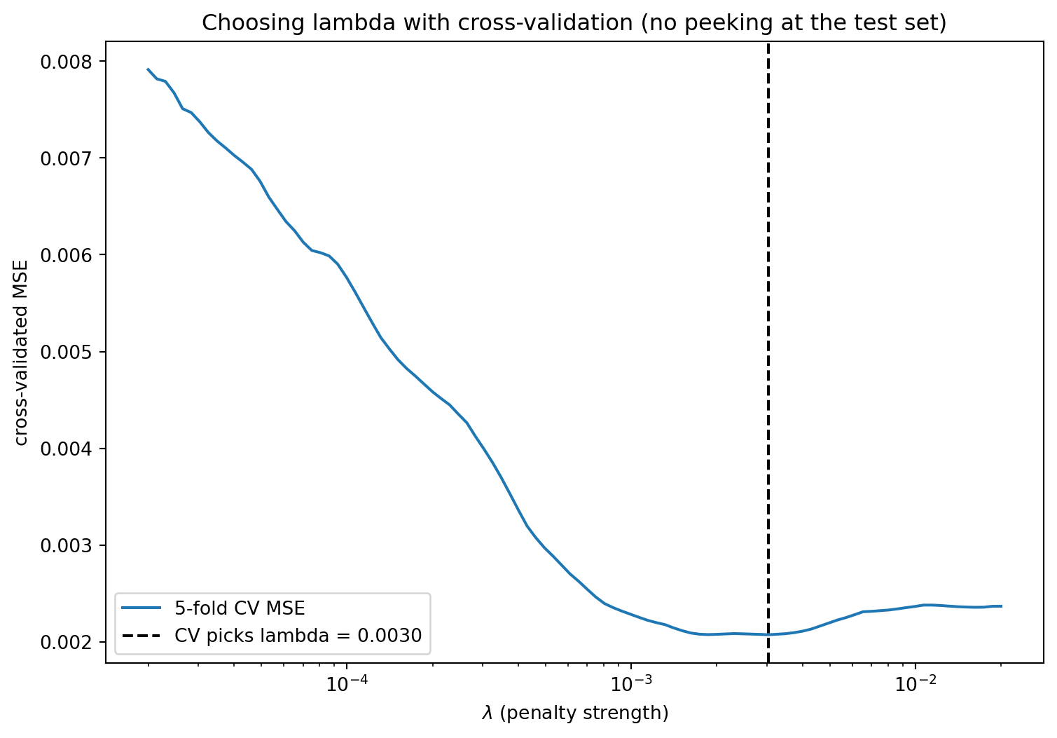
Only now, with \(\lambda\) chosen for each method, do we break the seal on the test set and compare all three models once. This is the same method which we learned in notebook 1.
results = pd.DataFrame({
    "model": ["OLS", "Ridge", "Lasso", "Predict the mean"],
    "test MSE": [
        mean_squared_error(y_test, ols.predict(X_test)),
        mean_squared_error(y_test, ridge.predict(X_test)),
        mean_squared_error(y_test, lasso.predict(X_test)),
        baseline_mse,
    ],
})
print(results.round(5).to_string(index=False))
model test MSE
OLS 0.03663
Ridge 0.00305
Lasso 0.00323
Predict the mean 0.00340OLS is far worse than predicting the mean. Ridge and lasso are both more than ten times better than OLS, lasso doing it with 14 variables and ridge with all 61. You have run the same recipe as Notebook 1, with \(\lambda\) in the role \(k\) played there.
The standard machine-learning recipe
Every later notebook in this stream reuses these four steps:
- Split off a test set and seal it away.
- Cross-validate on the training data to choose the hyperparameter.
- Pick the hyperparameter with the best CV score.
- Evaluate once on the sealed test set.
7. So have we found the effect of initial wealth on growth?
Lasso handed us a short list of variables, and gdpsh465, the country’s initial wealth, survived. That coefficient is the one the convergence question from section 1 turns on, so it is tempting to read the lasso coefficient on gdpsh465 as the causal answer to it.
It isn’t, and for more reasons which we didn’t go over in notebook 1. There are two more reasons specific to what we just did:
- The penalty biases coefficients on purpose. Lasso and ridge shrink every coefficient toward zero by design. That is a feature for prediction, where a little bias buys a lot of stability, but it is incorrect for estimation: the number on
gdpsh465is deliberately pulled toward zero, so it is not a clean estimate of anything. - Selecting controls and then reading off a coefficient is biased. We let lasso choose which controls to keep based on how well they predict growth. But a variable can be a weak predictor of growth and still be essential for de-confounding initial wealth, and lasso will drop these variables without a second thought. Choosing controls by predictive strength is not causal methodology.
That fix is post-double-selection lasso, and it is the subject of Notebook 5. A penalty tuned to predict growth well is not the same thing as a penalty that gives us an unbiased read on initial wealth, and techniques for remedying this are what the notebook stream is about.
Connections
- Back: Notebook 1 of this stream. There a single hyperparameter \(k\) traded bias against variance; here the penalty \(\lambda\) does the same, and the number of covariates is the flexibility which causes issues.
- Forward to Notebook 3: we stayed with linear models here. Next we go to nonparametric models with decision trees, random forests, and boosting, a different way to be flexible.
References
- The Barro-Lee growth data, distributed with the
hdmR package and the Applied Causal Inference book repository (causalml-book.org). - Belloni, A., Chernozhukov, V., & Hansen, C. (2014). High-dimensional methods and inference on structural and treatment effects. Journal of Economic Perspectives, 28(2), 29-50. The growth application and the double-selection idea behind Notebook 5.
- GeeksforGeeks. (2025). Ridge regression vs lasso regression. GeeksforGeeks. https://www.geeksforgeeks.org/machine-learning/ridge-regression-vs-lasso-regression/
- Hoerl, A. E., & Kennard, R. W. (1970). Ridge regression: Biased estimation for nonorthogonal problems. Technometrics, 12(1), 55-67.
- James, G., Witten, D., Hastie, T., & Tibshirani, R. (2021). An Introduction to Statistical Learning. Springer. (Chapter 6.)
- Murel, J., & Kavlakoglu, E. (n.d.). What is ridge regression? IBM. https://www.ibm.com/think/topics/ridge-regression
- Tibshirani, R. (1996). Regression shrinkage and selection via the lasso. Journal of the Royal Statistical Society: Series B, 58(1), 267-288.
- Wikipedia contributors. (n.d.). Lasso (statistics). Wikipedia. https://en.wikipedia.org/wiki/Lasso_(statistics)