import numpy as np
import pandas as pd
import matplotlib.pyplot as plt

from sklearn.linear_model import LogisticRegression, LinearRegression
from sklearn.preprocessing import StandardScaler

RANDOM_STATE = 42
TRUE_EFFECT = 2.0 # used later, in a simulated world where we set the real effect ourselvesPropensity Scores and Doubly-Robust Estimation
Python
machine learning
causal inference
propensity score
inverse probability weighting
treatment effects
The sixth notebook in the Causal ML stream. We return to the 401(k) question and adjust for confounders a second way: by modelling who gets treated. We estimate the propensity score, reweight the data with inverse probability weighting, and combine the treatment model with the outcome model into the doubly-robust estimator
Outline
Prerequisites
- Notebook 5 of this stream: estimating a treatment effect by adjusting for confounders
- Comfort with
pandasand basic Python at the COMET-intermediate level
Learning Outcomes
By the end of this notebook you will be able to:
- Define the propensity score and estimate it from data.
- Explain and compute inverse probability weighting (IPW).
- Read a covariate-balance plot and say what weighting does to the data.
- Explain why the outcome route and the treatment route each fail when their model is wrong.
- Compute the doubly-robust (AIPW) estimator and explain what “doubly robust” means.
1. Two routes to the same effect
Notebook 4 left us with a recipe for the effect of 401(k) eligibility on savings. Using the unconfoundedness assumption, comparing eligible and ineligible households that match on their characteristics \(X\) recovers the effect. We did this by modeling the outcome: predict savings from eligibility and \(X\), then read off the difference. That was one of our two routes.
In this notebook, instead of modelling savings, we model who gets treated. If we can work out each household’s chance of being eligible given its characteristics, we can use that chance to undo the imbalance between the two groups. You can look at this like the opposite of notebook 4, instead of modelling savings we model eligibility. The chance of treatment given \(X\) is called the propensity score, and it leads to two estimators, inverse probability weighting and the doubly-robust estimator, that we build here.
Both routes aim at the same number, the average effect of eligibility.
2. The Propensity Score
The propensity score is the probability of being treated given the covariates, \(e(X) = P(D = 1 \mid X)\). For our data it is the chance that a household with a given age, income, education, etc, is eligible for a 401(k). We don’t know this for certain as we can’t directly see it in our real data, so we will estimate it, this is a yes/no question so we will use a logistic regression.
savings = pd.read_csv("datasets/Pension401k.csv")
confounders = ["age", "inc", "educ", "fsize", "marr", "twoearn", "db", "pira", "hown"]
D = savings["e401"].to_numpy()        # treatment: eligible for a 401(k)
Y = savings["net_tfa"].to_numpy()     # outcome: net financial assets
X = savings[confounders].to_numpy()
X_std = StandardScaler().fit_transform(X)

propensity = LogisticRegression(max_iter=2000).fit(X_std, D).predict_proba(X_std)[:, 1]
print(f"Propensity score ranges from {propensity.min():.2f} to {propensity.max():.2f}")
print(f"Share of households eligible: {D.mean():.2f}")
Propensity score ranges from 0.10 to 0.98
Share of households eligible: 0.37For a comparison to be possible everywhere, both eligible and ineligible households have to appear at every propensity value. This is the overlap or positivity condition from Notebook 4.
The visualization below shows the overlap condition, both ineligible and eligible households appear across the whole range, so a comparison is possible.
plt.figure(figsize=(9, 5))
plt.hist(propensity[D == 0], bins=30, alpha=0.6, density=True, label="ineligible")
plt.hist(propensity[D == 1], bins=30, alpha=0.6, density=True, label="eligible")
plt.xlabel("estimated propensity score (chance of being eligible)")
plt.ylabel("density")
plt.title("Both groups appear across the whole range, so a comparison is possible")
plt.legend()
plt.show()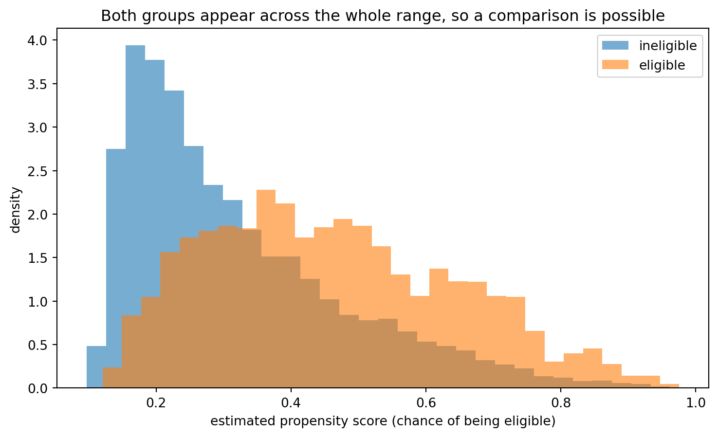
Both curves cover the range from near zero to near one. Every household has comparable households on the other side, so overlap holds and we can proceed.
2.1 Inverse probability weighting
For inverse probability weighting we take an eligible household that, given its characteristics, was unlikely to be eligible, meaning it has a low propensity score. It is rare among the eligible, and it stands in for many similar households that ended up ineligible. So we let it count for more, giving it a weight of one over its propensity, \(1/e(X)\). We do the mirror image on the other side, weighting each ineligible household by one over its chance of being ineligible, \(1/(1 - e(X))\). After this reweighting the two groups carry the same spread of characteristics, as though eligibility had been handed out at random.
We can watch the reweighting work. For each covariate, measure how far apart the eligible and ineligible groups are, before weighting and after.
e = np.clip(propensity, 0.01, 0.99)   # clip extremes so we never divide by a near-zero number
w = np.where(D == 1, 1 / e, 1 / (1 - e))

before, after = [], []
for j in range(len(confounders)):
    v = X[:, j]
    before.append((v[D == 1].mean() - v[D == 0].mean()) / v.std())
    tw = np.sum(w[D == 1] * v[D == 1]) / np.sum(w[D == 1])
    cw = np.sum(w[D == 0] * v[D == 0]) / np.sum(w[D == 0])
    after.append((tw - cw) / v.std())

rows = np.arange(len(confounders))
plt.figure(figsize=(8, 6))
plt.scatter(np.abs(before), rows, color="tab:red", zorder=3, label="before weighting")
plt.scatter(np.abs(after), rows, color="tab:green", zorder=3, label="after weighting")
plt.axvline(0, color="black", linewidth=0.8)
plt.yticks(rows, confounders)
plt.xlabel("gap between groups, in standard deviations (closer to 0 is better balanced)")
plt.title("Weighting by the propensity score balances the covariates")
plt.legend()
plt.show()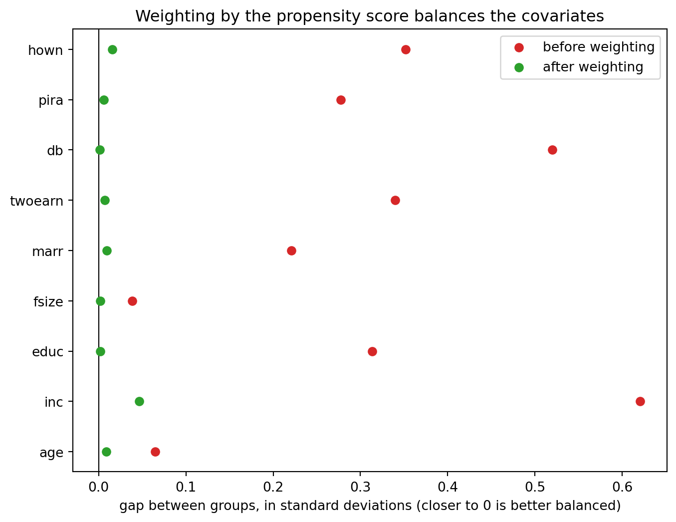
Before weighting, the red dots sit well away from zero: the eligible and ineligible groups differ on most characteristics, with income having the largest gap. After weighting, the green dots collapse toward zero. The groups now look alike. With them balanced, the inverse probability weighting (IPW) estimate of the effect is the difference between the weighted average savings of the two groups.
def ipw_ate(D, Y, e):
    treated = np.sum((D / e) * Y) / np.sum(D / e)
    control = np.sum(((1 - D) / (1 - e)) * Y) / np.sum((1 - D) / (1 - e))
    return treated - control

print(f"IPW estimate of the effect of eligibility: {ipw_ate(D, Y, e):.2f}")
IPW estimate of the effect of eligibility: 1.70On the 401(k) data this gives 1.7 thousand dollars. Notice it sits well below the outcome-route estimate from Notebook 4, which was 5.9 thousand. The two routes disagree, and so far we don’t have the tools to say which to believe. That is what will be discussed in the next section.
3. Our two routes and their different models
The outcome route is only as good as the savings model. If our prediction of savings given \(X\) is wrong, the estimate is biased. The treatment route, IPW, is only as good as the propensity model, so if our prediction of eligibility given \(X\) is wrong, the weights are wrong and so is the estimate. On real data we cannot see which model is off, because we never know the true effect, so as we did in the past, we will build a world where we do.
In this world the true effect is 2, we set it ourselves. Both the chance of treatment and the level of savings depend on a covariate through a squared term, so a model that includes that term is correct and a model that leaves it out is wrong. We can then hand each estimator a correct or a wrong model on purpose and see what happens.
def simulate(n, seed):
    rng = np.random.default_rng(seed)
    Xs = rng.normal(0, 1, (n, 4))
    index = 0.6 * Xs[:, 0] - 0.6 * Xs[:, 1] + 0.7 * Xs[:, 0] ** 2   # propensity depends on a square
    elig = (rng.uniform(size=n) < 1 / (1 + np.exp(-index))).astype(float)
    out = TRUE_EFFECT * elig + Xs[:, 0] + Xs[:, 1] + Xs[:, 0] ** 2 + rng.normal(0, 1, n)
    return Xs, elig, out

X_sim, D_sim, Y_sim = simulate(5000, RANDOM_STATE)
with_square = np.column_stack([X_sim, X_sim[:, 0] ** 2])   # the correct model includes the square
plain = X_sim                                              # the wrong model leaves it out

def fit_routes(X_out, X_ps):
    e = np.clip(LogisticRegression(max_iter=2000).fit(X_ps, D_sim).predict_proba(X_ps)[:, 1], 0.01, 0.99)
    mu1 = LinearRegression().fit(X_out[D_sim == 1], Y_sim[D_sim == 1]).predict(X_out)
    mu0 = LinearRegression().fit(X_out[D_sim == 0], Y_sim[D_sim == 0]).predict(X_out)
    return e, mu1, mu0

scenarios = [("both models right", with_square, with_square),
             ("outcome model wrong", plain, with_square),
             ("propensity model wrong", with_square, plain)]

print(f"true effect = {TRUE_EFFECT}")
for name, X_out, X_ps in scenarios:
    e_s, mu1_s, mu0_s = fit_routes(X_out, X_ps)
    print(f"  {name:24s}: regression {np.mean(mu1_s - mu0_s):.2f}   IPW {ipw_ate(D_sim, Y_sim, e_s):.2f}")
true effect = 2.0
both models right : regression 2.00 IPW 2.10
outcome model wrong : regression 2.78 IPW 2.10
propensity model wrong : regression 2.00 IPW 2.83When both models are right, both routes recover the true 2. When the outcome model is wrong, the regression route is biased (2.78) while IPW, still using the right propensity, is correct. When the propensity model is wrong, IPW is biased (2.83) while the regression route is correct. Each route fails when its own model fails, and on real data we would not know that it had happened.
4. The doubly-robust estimator
We want an estimator that survives a wrong model as long as the other one is right. The augmented inverse probability weighting (AIPW) estimator does this by using both at once.
Start with the outcome route’s answer, which is the regression estimate of the effect. Then check whether the outcome model actually fit: look at its mistakes, the gap between each household’s real savings and what the model predicted. Reweight those mistakes the IPW way and add them on as a correction. Written out, the estimate is the average over households of:
\[ \hat{\tau} = \frac{1}{n} \sum_{i} \Big[ \underbrace{\hat{\mu}_1(X_i) - \hat{\mu}_0(X_i)}_{\text{regression guess}} + \underbrace{\frac{D_i \, (Y_i - \hat{\mu}_1(X_i))}{e(X_i)} - \frac{(1 - D_i) \, (Y_i - \hat{\mu}_0(X_i))}{1 - e(X_i)}}_{\text{correction from the model's mistakes}} \Big] \]
Read this for the meaning, not the symbols
Do not try to follow the formula term by term. The only thing to hold onto is its shape: the first part is the regression guess of the effect, and the second part is a correction built from the outcome model’s mistakes, weighted like in the IPW.
What matters is what the correction does in each case:
- If the outcome model is right, it makes no systematic mistakes, so its residuals average to nothing and the correction vanishes. We keep the correct regression estimate.
- If the outcome model is wrong but the propensity is right, those mistakes are where the leftover bias is hiding, and weighting them like IPW is what removes it.
Either way the answer comes out right, as long as one of the two models is correct. This is very powerful when we can’t for certain tell if our model is right.
What “doubly robust” means
An estimator is doubly robust if it stays correct as long as at least one of its two models, the outcome model or the propensity model, is right, which gives you two chances instead of one. It does not save you if both models are wrong, and it does nothing about an unmeasured confounder, which breaks unconfoundedness itself and is beyond the reach of every estimator in this notebook.
We run all three estimators in our made-up example and plot them.
def aipw_score(D, Y, e, mu1, mu0):
    return mu1 - mu0 + D * (Y - mu1) / e - (1 - D) * (Y - mu0) / (1 - e)

labels, reg_vals, ipw_vals, aipw_vals = [], [], [], []
for name, X_out, X_ps in scenarios:
    e_s, mu1_s, mu0_s = fit_routes(X_out, X_ps)
    labels.append(name.replace(" ", "\n"))
    reg_vals.append(np.mean(mu1_s - mu0_s))
    ipw_vals.append(ipw_ate(D_sim, Y_sim, e_s))
    aipw_vals.append(np.mean(aipw_score(D_sim, Y_sim, e_s, mu1_s, mu0_s)))

pos = np.arange(len(labels))
plt.figure(figsize=(9, 5))
plt.bar(pos - 0.25, reg_vals, 0.25, label="regression", color="tab:blue")
plt.bar(pos, ipw_vals, 0.25, label="IPW", color="tab:orange")
plt.bar(pos + 0.25, aipw_vals, 0.25, label="AIPW (doubly robust)", color="tab:green")
plt.axhline(TRUE_EFFECT, color="black", linestyle="--", label=f"true effect = {TRUE_EFFECT:.0f}")
plt.xticks(pos, labels)
plt.ylabel("estimated effect")
plt.title("Only AIPW lands on the truth when one of the two models is wrong")
plt.legend()
plt.show()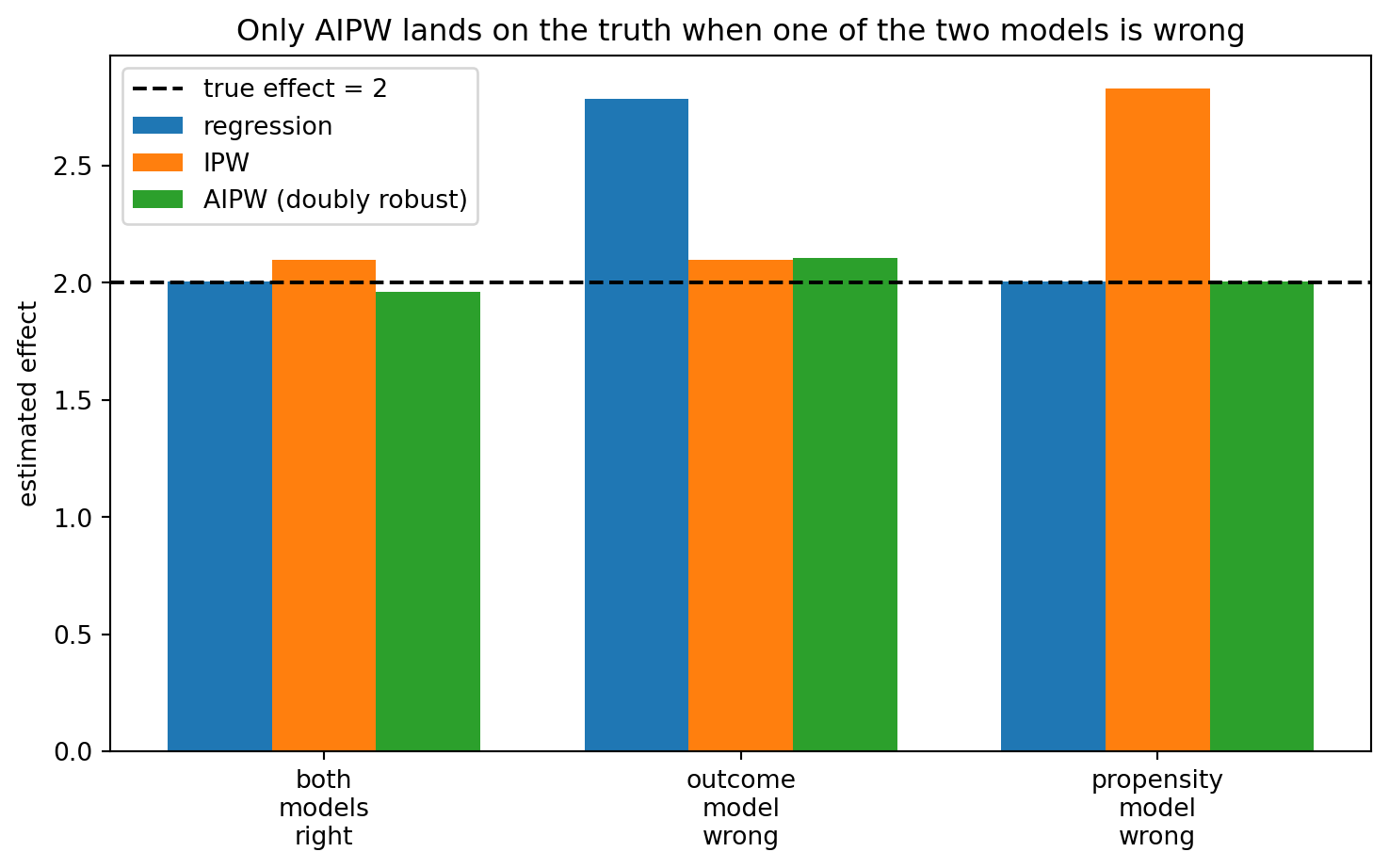
Regression (blue) is off when the outcome model is wrong; IPW (orange) is off when the propensity model is wrong; AIPW (green) sits on the true effect in all three worlds. It needed only one of its two models to be right.
4.1 The conditions that make these estimates causal
Before we take AIPW to the real data, we should collect all of the statistical conditions under which the numbers in this notebook, the IPW estimate and the AIPW estimate, identify a causal effect. The first two are the identification conditions from Notebook 4, the third is the sampling condition behind the standard errors, and the fourth is where the estimators in this notebook differ from one another.
Identification conditions for IPW and the doubly-robust estimator
- Unconfoundedness (selection on observables). The nine covariates must contain every systematic reason a household ends up eligible that also matters for its savings: \((Y(0), Y(1)) \perp D \mid X\). Both routes, modelling the outcome and modelling the treatment, adjust for the same \(X\), so both fail together if a confounder is missing from it. This assumption cannot be tested from the data.
- Overlap (positivity), and strictly so. Every kind of household must have a real chance of being both eligible and ineligible: \(0 < e(X) < 1\). For weighting this matters, because the weights are \(1/e(X)\) and \(1/(1-e(X))\), so a propensity near zero or one makes a single household dominate the estimate and the variance grow rapidly. That is why we clipped the scores; clipping stabilizes the weights, but frequent clipping is a warning that overlap is thin and the estimate rests on few comparable households.
- A random, independent sample and one version of treatment. The households are treated as i.i.d. draws from the population of interest, each household’s eligibility does not affect another household’s savings, and “eligible” means the same thing for everyone (together, the SUTVA and consistency conditions). The simple standard error we compute for AIPW leans on this independence.
- At least one correctly specified model. IPW additionally requires the propensity model to be right; the outcome route requires the savings model to be right. AIPW is the safety net between them: it identifies the effect if either the propensity model or the outcome model is correct. That is a weaker modelling requirement than either route alone, but it is not a guarantee; if both models are wrong, or if condition 1 fails, the doubly-robust estimate is biased too.
4.2 The doubly-robust estimate on the 401(k) data
We will apply the model to our real savings data, combining the logistic propensity from section 2 with simple linear models of savings.
mu1 = LinearRegression().fit(X_std[D == 1], Y[D == 1]).predict(X_std)
mu0 = LinearRegression().fit(X_std[D == 0], Y[D == 0]).predict(X_std)

score = aipw_score(D, Y, e, mu1, mu0)
aipw = score.mean()
aipw_se = score.std() / np.sqrt(len(score))
print(f"AIPW estimate: {aipw:.2f}  (se {aipw_se:.2f})")
print(f"95% interval : {aipw - 1.96 * aipw_se:.2f} to {aipw + 1.96 * aipw_se:.2f}")
AIPW estimate: 1.91 (se 3.55)
95% interval : -5.04 to 8.87The point estimate is 1.91 thousand dollars. The raw gap between eligible and ineligible households was about 19.6 thousand (Notebook 4), and AIPW puts the de-confounded effect near 1.9. Almost all of that raw gap was selection: eligible households were already richer savers, and once we account for that, what looked like a $19,600 effect is at most a couple of thousand (look at the upper bound of the 95% confidence interval). We have shown that shrinkage (selection bias), which is an important lesson in this notebook on real data.
What we cannot yet do is measure the piece that is left precisely. The standard error is large (3.55), and the 95% interval contains large negative values, zero and large positive values, so we cannot even be sure the effect is positive. Savings are very spread out, a few households hold enormous amounts, and reweighting a quantity like that is noisy. Simple linear models remove the bias but leave too much variance behind. We will close this gap in the next notebook which is double machine learning.
Self-test
Suppose you are confident your propensity model is right but unsure about your outcome model. Does AIPW help you, and how?
Show / hide answer
Yes. AIPW is correct as long as either model is right, so a correct propensity model alone is enough to make the estimate consistent, whatever the outcome model does. In that case AIPW behaves like a refined version of IPW: the outcome model is along for the ride and mostly reduces the variance. The same holds with the roles reversed, and that is the appeal of having two chances.5. Connections
This notebook added the treatment-modelling route to the outcome-modelling route of Notebook 4, and combined them. The combination, AIPW, is the bridge to the rest of the stream: its score is the object that double machine learning (notebook 7) is built around.
- Back to Notebook 5: there we adjusted for confounders by selecting controls for a single regression; here we adjust by modelling the treatment instead, and then combine the two routes.
- Forward to Notebook 7: double machine learning, which estimates the two models with any learner and computes the doubly-robust score with cross-fitting, turning this notebook’s noisy estimate into a sharp one.
References
- Chernozhukov, V., Chetverikov, D., Demirer, M., Duflo, E., Hansen, C., Newey, W., & Robins, J. (2018). Double/debiased machine learning for treatment and structural parameters. Econometrics Journal, 21(1), C1-C68. The cross-fitting that Notebook 7 builds on.
- Facure, M. (2023). Doubly robust estimation (Chapter 12). In Causal Inference for the Brave and True. https://matheusfacure.github.io/python-causality-handbook/12-Doubly-Robust-Estimation.html
- Glynn, A., & Quinn, K. (2009). An Introduction to the Augmented Inverse Propensity Weighted Estimator. https://www.law.berkeley.edu/archive/files/AIPW(1).pdf
- Poterba, J. M., Venti, S. F., & Wise, D. A. (1995). Do 401(k) contributions crowd out other personal saving? Journal of Public Economics, 58(1), 1-32. The eligibility question.
- Robins, J. M., Rotnitzky, A., & Zhao, L. P. (1994). Estimation of regression coefficients when some regressors are not always observed. Journal of the American Statistical Association, 89(427), 846-866. The augmented, doubly-robust estimator.
- Rosenbaum, P. R., & Rubin, D. B. (1983). The central role of the propensity score in observational studies for causal effects. Biometrika, 70(1), 41-55.