import numpy as np
import pandas as pd
import matplotlib.pyplot as plt

from sklearn.linear_model import LassoCV, LogisticRegression
from sklearn.ensemble import (RandomForestRegressor, RandomForestClassifier,
                              GradientBoostingRegressor, GradientBoostingClassifier,
                              ExtraTreesRegressor)
from sklearn.model_selection import KFold

RANDOM_STATE = 42Double Machine Learning
Python
machine learning
causal inference
double machine learning
cross-fitting
treatment effects
The seventh notebook in the Causal ML stream. We combine everything: the partially linear model, the residual-on-residual idea from Notebook 4, and any learner we like for the nuisance models. We add cross-fitting to stop the learners from contaminating the estimate, attach a standard error, and finally pin down the effect of 401(k) eligibility that Notebook 6 left as a wide interval.
Outline
Prerequisites
- Notebook 6 of this stream: estimating a treatment effect, and why a wide confidence interval leaves us stuck
- Multiple regression and the idea of partialling out controls (COMET Intermediate)
- Comfort with
pandasand basic Python at the COMET-intermediate level
Learning Outcomes
By the end of this notebook you will be able to:
- Write down the partially linear model and identify the treatment effect in it.
- Estimate that effect by residual-on-residual regression with any learner.
- Explain why fitting the learners and the effect on the same data biases the estimate, and fix it with cross-fitting.
- Run a full double machine learning estimate with a standard error.
- Swap in any learner and see the estimate hold.
1. Where we Currently Stand After Notebook 6
The last three notebooks approached the same problem from different angles. Notebook 4 removed the controls from the outcome and the treatment separately, then regressed on the leftovers (orthogonalization). Notebook 5 did this for lasso, selecting controls twice. Notebook 6 modelled the treatment and combined the two routes into the doubly-robust estimator. Notebook 6 also left us stuck: its estimate of the 401(k) effect was 1.9 thousand dollars, but with a confidence interval running from negative five up to about positive nine, far too wide to tell whether eligibility helped at all. It was imprecise.
This notebook closes that gap. Double machine learning (DML) keeps the residual-on-residual concept from before and adds two things which greatly increase its power and usefulness:
- Any learner. A learner is any prediction algorithm that fits a function to data, the kind of model we built in Notebooks 1 to 3. The two models we fit along the way, savings given the covariates and treatment given the covariates, are prediction problems, so we can use whichever learner predicts best: a lasso, a random forest, a boosted ensemble, a neural network or anything else that fits the data.
- Cross-fitting. A method that stops our new flexible learners from biasing the effect, built from the train/test idea of Notebook 1.
DML will lead to a sharp, significant estimate of the effect of 401(k) eligibility on savings.
2. The partially linear model
To say what we are estimating, we write down a model. The partially linear model splits the outcome into the part we care about and the part we do not:
\[ Y = \theta D + g(X) + \varepsilon . \]
Here \(Y\) is savings, \(D\) is eligibility, and \(X\) is the covariates. The number \(\theta\) is the effect of eligibility, the one thing we want. The function \(g(X)\) is everything else that drives savings: income, age, and any other controls, and it can take any shape. The treatment depends on the covariates too:
\[ D = m(X) + v . \]
The function \(m(X)\) is the propensity from Notebook 6, the part of eligibility explained by the covariates, and \(v\) is what is left.
Read these for the meaning
\(g\) and \(m\) are called nuisance functions: we have to estimate them well, but we don’t care what they are. We just want a clean value of \(\theta\) while the messy functions \(g\) and \(m\) are handled by a learner in the background. The word “linear” in the name refers only to how \(D\) enters, through a single number \(\theta\). Everything else, \(g(X)\), can be nonlinear.
2.1 Orthogonalization: residual on residual
The trick for isolating \(\theta\) is the one we used in Notebook 4: remove the covariates’ influence out of both sides, and then compare what is left. The covariates \(X\) are the confounders, the common causes of eligibility and savings, so removing them from both the outcome and the treatment cleans the comparison.
Predicting savings from the covariates and subtracting leaves \(\tilde{Y} = Y - g(X)\), the part of savings the covariates do not explain. Doing the same for eligibility leaves \(\tilde{D} = D - m(X)\), the part of eligibility the covariates do not explain. Subtracting \(g(X)\) from the model leaves
\[ \tilde{Y} = \theta \tilde{D} + \varepsilon , \]
so the slope of \(\tilde{Y}\) on \(\tilde{D}\) is exactly \(\theta\). This is a famous result from Econometrics called the Frisch-Waugh-Lovell theorem. It states that multivariate regression coefficients can be calculated by “partialling out” (or residualizing) the influence of control variables from both the dependent variable and the primary independent variables. Residualizing first and controlling for everything at once are two roads to the same number. Notebook 4 demonstrated the first road with a lasso doing the predicting. The new freedom in DML is that any learner can play the role of \(g\) and \(m\), since we just need them to predict well.
There is one catch, the same one from Notebook 1: we can’t use the same data twice.
2.2 The issue with fitting and estimating on the same data
Suppose we fit the two learners and compute the effect all on the same households. The danger is overfitting, a core theme of Notebooks 1, 2, and 3. A flexible learner can fit the training data too well, memorizing the noise and not being able to generalize to new data. If we feed these overfitting estimators into the residual-on-residual regression the effect comes out wrong.
We will make this happen on purpose to demonstrate it. We build a world where the true effect is 1, and we hand the residualizing to a learner that memorises its training data and dramatically overfits: an extremely-randomised forest grown until every household sits in its own leaf. On the training data it predicts perfectly, so the leftovers collapse to nothing.
def make_world(n, seed):
    rng = np.random.default_rng(seed)
    X = rng.normal(0, 1, (n, 8))
    g = X[:, 0] + 0.7 * X[:, 1] + 0.5 * X[:, 2] + 0.4 * X[:, 0] * X[:, 1]
    m = 0.6 * X[:, 0] + 0.4 * X[:, 2]
    D = m + rng.normal(0, 1, n)
    Y = 1.0 * D + g + rng.normal(0, 1, n)   # the true effect is 1
    return X, D, Y

X_sim, D_sim, Y_sim = make_world(1000, RANDOM_STATE)

def memoriser():
    return ExtraTreesRegressor(n_estimators=100, min_samples_leaf=1,
                               bootstrap=False, random_state=RANDOM_STATE, n_jobs=-1)

# Same data for fitting and for the effect: no cross-fitting.
y_leftover = Y_sim - memoriser().fit(X_sim, Y_sim).predict(X_sim)
d_leftover = D_sim - memoriser().fit(X_sim, D_sim).predict(X_sim)
theta_same_data = np.sum(d_leftover * y_leftover) / np.sum(d_leftover * d_leftover)

print(f"Leftover spread on the training data: Y {y_leftover.std():.3f}, D {d_leftover.std():.3f}")
print(f"Effect estimated on the same data: {theta_same_data:.2f}  (true effect is 1.0)")
Leftover spread on the training data: Y 0.000, D 0.000
Effect estimated on the same data: -0.10 (true effect is 1.0)The leftovers are approaching zero, because the learner reads the training outcomes back to us, memorizing the noise not true predictive signal. With nothing left to regress, the estimate collapses to -0.10, nowhere near the true 1.
The fix is cross-fitting, and it is the train/test split of Notebook 1 applied to the nuisance models. Split the data into folds. To get a household’s leftover, use a learner that was fit on the other folds, never on that household. A learner can’t memorise a household it was not shown, so the leftovers keep their real spread.
def crossfit_leftovers(X, target, make_model, n_splits=5):
    leftover = np.zeros(len(target))
    folds = KFold(n_splits, shuffle=True, random_state=RANDOM_STATE)
    for train_idx, test_idx in folds.split(X):
        model = make_model().fit(X[train_idx], target[train_idx])
        leftover[test_idx] = target[test_idx] - model.predict(X[test_idx])
    return leftover

y_cf = crossfit_leftovers(X_sim, Y_sim, memoriser)
d_cf = crossfit_leftovers(X_sim, D_sim, memoriser)
theta_crossfit = np.sum(d_cf * y_cf) / np.sum(d_cf * d_cf)
print(f"Effect estimated with cross-fitting: {theta_crossfit:.2f}  (true effect is 1.0)")
Effect estimated with cross-fitting: 0.93 (true effect is 1.0)With cross-fitting the estimate is 0.93, close to the true value of 1. The plot lines the two up against the truth.
plt.figure(figsize=(7, 5))
plt.bar(["same data\n(no cross-fitting)", "cross-fitting"],
        [theta_same_data, theta_crossfit],
        color=["tab:red", "tab:green"])
plt.axhline(1.0, color="black", linestyle="--", label="true effect = 1")
plt.ylabel("estimated effect")
plt.title("Cross-fitting rescues the estimate from a memorising learner")
plt.legend()
plt.show()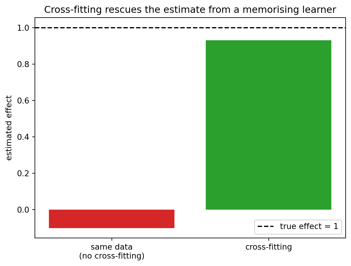
The cross-fitting rule
Never use the same household both to fit a nuisance model and to compute its leftover. Fit on one part of the data, take leftovers on another, and rotate. This lets us add a flexible, non-overfitting learner into the procedure keeping the true effect uncontaminated. Orthogonalization plus cross-fitting is what makes the name double machine learning.
3. Double Machine Learning
We now have every piece. The recipe: cross-fit the leftovers of the outcome and the treatment with whatever learner we choose, then regress one on the other for the effect. A standard error comes from the spread of the per-household terms, the same influence-function concept from the doubly-robust score in Notebook 6.
def dml_effect(X, D, Y, make_outcome, make_treatment, n_splits=5):
    folds = KFold(n_splits, shuffle=True, random_state=RANDOM_STATE)
    y_left = np.zeros(len(Y))
    d_left = np.zeros(len(D))
    for train_idx, test_idx in folds.split(X):
        out = make_outcome().fit(X[train_idx], Y[train_idx])
        y_left[test_idx] = Y[test_idx] - out.predict(X[test_idx])
        treat = make_treatment().fit(X[train_idx], D[train_idx])
        d_hat = treat.predict_proba(X[test_idx])[:, 1] if hasattr(treat, "predict_proba") \
            else treat.predict(X[test_idx])
        d_left[test_idx] = D[test_idx] - d_hat
    theta = np.sum(d_left * y_left) / np.sum(d_left * d_left)
    resid = y_left - theta * d_left
    se = np.sqrt(np.mean(d_left ** 2 * resid ** 2) / np.mean(d_left ** 2) ** 2 / len(Y))
    return theta, se
Now we load our real 401(k) data and run it, using a random forest to model both savings and eligibility.
savings = pd.read_csv("datasets/Pension401k.csv")
confounders = ["age", "inc", "educ", "fsize", "marr", "twoearn", "db", "pira", "hown"]
D = savings["e401"].to_numpy().astype(float)
Y = savings["net_tfa"].to_numpy()
X = savings[confounders].to_numpy()

def forest_reg():
    return RandomForestRegressor(n_estimators=300, min_samples_leaf=20,
                                 random_state=RANDOM_STATE, n_jobs=-1)
def forest_clf():
    return RandomForestClassifier(n_estimators=300, min_samples_leaf=20,
                                  random_state=RANDOM_STATE, n_jobs=-1)

theta, se = dml_effect(X, D, Y, forest_reg, forest_clf)
print(f"DML estimate of the effect of eligibility: {theta:.2f}  (se {se:.2f})")
print(f"t-statistic: {theta / se:.1f}")
print(f"95% interval: {theta - 1.96 * se:.2f} to {theta + 1.96 * se:.2f}")
DML estimate of the effect of eligibility: 8.80 (se 1.35)
t-statistic: 6.5
95% interval: 6.15 to 11.45The effect is 8.80 thousand dollars, with a standard error of 1.35 and a t-statistic of 6.5. The 95% interval runs from 6.15 to 11.45, well clear of zero. Eligibility for a 401(k) raised net financial assets by 8,800 dollars. This is the number Notebook 6 could not reach: its interval reached up toward nine but could not rule out zero, and DML, with flexible models and cross-fitting, finds the positive effect. Most of the raw 19.6 gap from Notebook 4 was selection, but a real and substantial effect of 8,800 dollars remains underneath.
The picture behind the number is the residual-on-residual scatter, the same one from Notebook 4, now with the forest doing the residualizing. We compute the two leftovers out-of-fold and plot one against the other; the slope of the line is the effect.
folds = KFold(5, shuffle=True, random_state=RANDOM_STATE)
y_left = np.zeros(len(Y))
d_left = np.zeros(len(D))
for train_idx, test_idx in folds.split(X):
    y_left[test_idx] = Y[test_idx] - forest_reg().fit(X[train_idx], Y[train_idx]).predict(X[test_idx])
    treat = forest_clf().fit(X[train_idx], D[train_idx])
    d_left[test_idx] = D[test_idx] - treat.predict_proba(X[test_idx])[:, 1]

plt.figure(figsize=(8, 5))
plt.scatter(d_left, np.clip(y_left, -100, 200), s=6, alpha=0.2, color="grey")
grid = np.array([d_left.min(), d_left.max()])
plt.plot(grid, theta * grid, color="tab:green", linewidth=2, label=f"slope = {theta:.2f}")
plt.xlabel("leftover eligibility (after removing the covariates)")
plt.ylabel("leftover savings (after removing the covariates)")
plt.title("The effect is the slope through the residual-on-residual cloud")
plt.legend()
plt.show()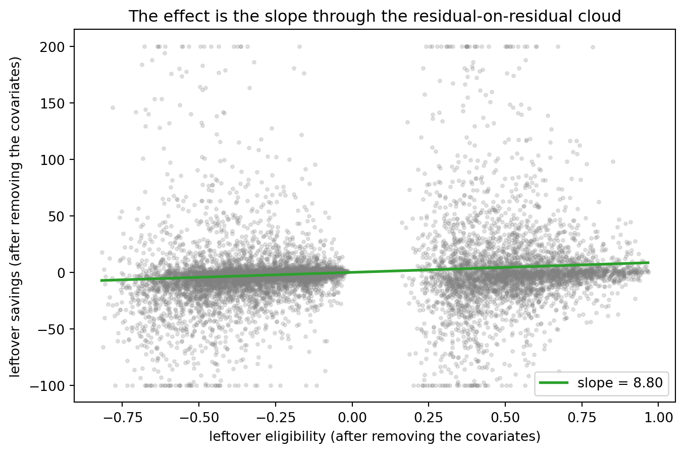
Each grey dot is one household, placed by how much of its eligibility and its savings is left once the covariates are stripped out. The cloud tilts upward: households with more leftover eligibility tend to have more leftover savings. The slope of that tilt, drawn in green, is the estimated effect of 8.80. It is the same residual-on-residual picture as Notebook 4, with a random forest doing the stripping in place of a lasso.
3.1 Any learner in DML
The causal machinery, residualize, cross-fit and regress, never mentioned which learner we used. So we can drop in any learner and the estimate holds. We run the same DML with three very different learners, a lasso, a random forest, and gradient boosting (the sequential tree method from Notebook 3, which builds many small models that each correct the errors left by the ones before).
learners = {
    "lasso": (lambda: LassoCV(cv=5, random_state=RANDOM_STATE, max_iter=50000),
              lambda: LogisticRegression(max_iter=2000)),
    "random forest": (forest_reg, forest_clf),
    "boosting": (lambda: GradientBoostingRegressor(random_state=RANDOM_STATE),
                 lambda: GradientBoostingClassifier(random_state=RANDOM_STATE)),
}

results = {name: dml_effect(X, D, Y, mo, mt) for name, (mo, mt) in learners.items()}
for name, (th, s) in results.items():
    print(f"{name:14s}: {th:.2f}  (se {s:.2f}, t {th / s:.1f})")
lasso : 6.12 (se 1.47, t 4.2)
random forest : 8.80 (se 1.35, t 6.5)
boosting : 9.62 (se 1.34, t 7.2)names = list(results)
thetas = [results[n][0] for n in names]
errs = [1.96 * results[n][1] for n in names]
plt.figure(figsize=(8, 5))
plt.bar(names, thetas, yerr=errs, capsize=6, color=["tab:blue", "tab:green", "tab:orange"])
plt.axhline(0, color="black", linewidth=1)
plt.ylabel("estimated effect of eligibility ($1,000s)")
plt.title("Any learner gives a positive, significant effect")
plt.show()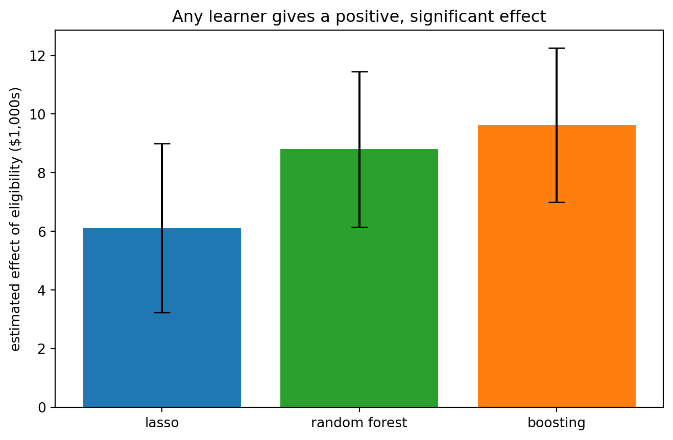
All three learners agree: the effect is positive and significant. The lasso, a linear model, finds 6.12; the random forest gives 8.80 and gradient boosting 9.62, both higher because they capture more of the tangled savings function. The exact number shifts with how flexibly we model the nuisances, but the end result does not. It is positive and significant!
Self-test
Cross-fitting splits the data into folds, much like the cross-validation of Notebook 1. Are they doing the same job?
Show / hide answer
No, they share the mechanism but not the purpose. Cross-validation in Notebook 1 splits the data to choose a hyperparameter, by scoring predictions on held-out folds. Cross-fitting splits the data to keep the nuisance models from contaminating the effect, by computing each household’s leftover from a model that never saw it.3.2 Review of the DML recipe
We built double machine learning a piece at a time. Here is the whole workflow gathered together:
The double machine learning recipe
- Pick the target. Write the partially linear model and identify the number you want, the treatment effect \(\theta\).
- Choose two learners. One to predict the outcome from the covariates, one to predict the treatment from the covariates. Any learner works, so pick whatever fits the data best.
- Cross-fit the leftovers. Split the data into folds. For each fold, fit both learners on the other folds and take each unit’s leftover, its value minus the prediction, out-of-fold, so no unit helps fit the model that later judges it.
- Regress leftover on leftover. Regress the outcome leftovers on the treatment leftovers. The slope is the estimated effect.
- Report the uncertainty. Take the standard error from the spread of the per-unit terms, and form the confidence interval.
3.3 The conditions that make the estimate causal
The recipe tells you how to compute the estimate, but by itself it does not make the estimate causal. The estimate of 8,800 dollars, and the confidence interval around it, identify the effect of eligibility only under the following statistical conditions. The first three are about the world and the data and are shared with Notebooks 4 to 6; the last two are the requirements DML places on its own machinery.
Identification conditions for double machine learning
- Unconfoundedness (selection on observables). The nine covariates must capture every systematic reason a household is eligible that also matters for savings. In the partially linear model this is carried by the error terms: \(\varepsilon\) and \(v\) must average to zero given the covariates, so that once \(g(X)\) and \(m(X)\) are removed, the leftover eligibility \(\tilde{D}\) is as good as random. Flexible learners make the adjustment for \(X\) better; they do nothing about a confounder that is not in \(X\), and this condition remains untestable.
- Overlap. The treatment must truly vary within every kind of household, so the leftover \(\tilde{D} = D - m(X)\) has spread everywhere. If the covariates predicted eligibility perfectly for some households, their \(\tilde{D}\) would collapse to zero and there would be nothing to regress on.
- A random, independent sample. The method for standard errors and cross-fitting treats households as i.i.d. draws, with no household’s eligibility affecting another household’s savings and a single version of the treatment (SUTVA and consistency).
- The partially linear model, with a constant effect. We wrote \(Y = \theta D + g(X) + \varepsilon\), so \(\theta\) is one number for everyone. Nonlinearity is allowed anywhere in \(g(X)\) and \(m(X)\), but not in how \(D\) enters. If the effect actually varies across households, the DML slope estimates a particular variance-weighted average of those effects rather than the plain ATE, and Notebook 8 looks at that heterogeneity directly.
- Nuisance learners that are good enough, plus orthogonalization and cross-fitting. The learners for \(g\) and \(m\) do not have to be perfect, but they must converge to the truth relatively well: the rule of thumb from the theory is that each should have an error shrinking at roughly the rate \(n^{-1/4}\), so the product of the two errors shrinks faster than \(1/\sqrt{n}\). Given that, the residual-on-residual (Neyman-orthogonal) construction makes the estimate insensitive to the small errors that remain, and cross-fitting removes the contamination from overfitting we demonstrated in Section 2.2. Skip the cross-fitting, or use a learner too weak to learn the nuisances at that rate, and the guarantee behind the standard error breaks.
Conditions 1 to 3 can’t be fixed with a stronger learner; conditions 4 and 5 are necessary for using flexible machine learning inside a causal estimate. When you report a DML effect, these five are the statement of what the causal claim rests on.
4. Connections
This notebook is where we see the stream’s biggest conceptual payoffs. The prediction tools from Notebooks 1 to 3 became the learners which power DML and the orthogonalization of Notebook 4 became the framework, and then cross-fitting made the technique trustworthy. The result is a recipe that estimates a causal effect with any learner and reports a valid standard error. In practice the doubleml python package implements all of this and more, but the moving parts are the ones we built by hand here.
- Back to Notebook 6: there the doubly-robust estimate of the 401(k) effect was too imprecise to sign; double machine learning sharpens it to about 9,000 dollars by using flexible learners and cross-fitting.
- Forward to Notebook 8: from the average effect to who benefits, estimating effects that vary across households with causal forests.
References
- Ahrens, A., Chernozhukov, V., Hansen, C., Kozbur, D., Schaffer, M., & Wiemann, T. (2025). An introduction to double/debiased machine learning. arXiv:2504.08324.
- Bach, P., Chernozhukov, V., Kurz, M. S., & Spindler, M. (2022). DoubleML: An object-oriented implementation of double machine learning in Python. Journal of Machine Learning Research, 23(53), 1-6.
- Chernozhukov, V., Chetverikov, D., Demirer, M., Duflo, E., Hansen, C., Newey, W., & Robins, J. (2018). Double/debiased machine learning for treatment and structural parameters. Econometrics Journal, 21(1), C1-C68. The orthogonal moment and cross-fitting.
- Frisch, R., & Waugh, F. V. (1933). Partial time regressions as compared with individual trends. Econometrica, 1(4), 387-401. The residual-on-residual result.
- Poterba, J. M., Venti, S. F., & Wise, D. A. (1995). Do 401(k) contributions crowd out other personal saving? Journal of Public Economics, 58(1), 1-32. The eligibility question.