import os
import time
import sqlite3
import duckdb
import numpy as np
import pandas as pdStorage, Speed, and Transactions
Python
SQL
data engineering
The sixth notebook in the Data Engineering stream. Before wave 2 of the survey goes live, the survey office wants proof the system works. We take manual control of transactions and crash the database on purpose, make a lookup about thirty times faster with an index, and race SQLite against DuckDB to see why analytics reads columns.
Outline
Prerequisites
- Notebook 5 of this stream: the designed schema.
Learning Outcomes
By the end of this notebook you will be able to:
- Control a transaction with
BEGIN,COMMITandROLLBACK, and undo a mistake. - Explain ACID, and demonstrate atomicity, isolation and durability with a crash we cause on purpose.
- Make a slow query fast with an index, prove what changed with EXPLAIN QUERY PLAN, and state what the speed costs.
- Explain row and column storage, and predict which type of workloads each one wins.
- Justify Parquet over CSV for data you keep.
1. Where we are in the stream
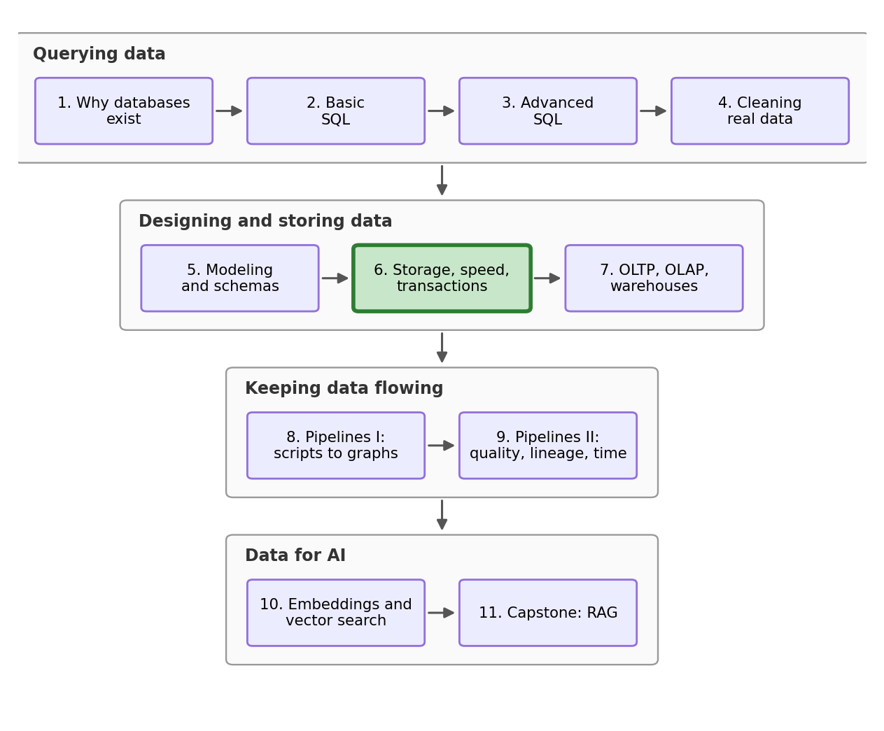
Notebook 5’s design was accepted, and the survey office is building the wave 2 intake software with it. The schema tells us what a valid record is. We also received a new email from the survey office for this notebook’s task.
The launch review, from the survey office. “Three questions before we sign off. One: interviewers’ laptops have died mid-interview in the past, so tell us what a crash does to the data. Two: looking up a respondent’s history has to stay instant once this thing holds years of responses. Three: the research side wants analytics on the archive without waiting all day, and wants to know what file format we keep the history in.”
Three questions, and in this notebook we answer each with an experiment (fun)! Along the way we meet the mechanism beneath everything this stream has done so far: how a database writes without losing data, how it finds one row without reading them all, and how the same data can sit on disk in shapes whose speed differs a hundredfold.
2. A quarter of a million rows
Every experiment today needs something the 1,000-row survey cannot give us: enough data for speed to matter. So we simulate the amount: two years of wave 2 operation, 250,000 interview responses, 250 times the survey we have been using so far. The grain is one row per response, and the same person can appear many times, once per interview they gave.
numpy’s random generator does the manufacturing. default_rng(42) builds a generator with a fixed seed, so every run of this notebook produces the identical dataset.
rng = np.random.default_rng(42)
n = 250_000

provinces = ["Ontario", "Quebec", "British Columbia", "Alberta", "Manitoba", "Saskatchewan"]
weights = [0.42, 0.23, 0.15, 0.13, 0.04, 0.03]
industries = ["Construction", "Education", "Finance", "Health care", "Hospitality",
              "Manufacturing", "Public administration", "Retail", "Technology"]

big = pd.DataFrame({
    "response_id": np.arange(1, n + 1),
    "respondent_id": rng.integers(1, 60_001, n),
    "interview_date": pd.Timestamp("2026-09-01") + pd.to_timedelta(rng.integers(0, 730, n), unit="D"),
    "province": rng.choice(provinces, n, p=weights),
    "industry": rng.choice(industries, n),
    "age": rng.integers(19, 66, n),
    "weekly_hours": rng.normal(37, 6, n).clip(5, 80).round(1),
    "hourly_wage": rng.lognormal(3.6, 0.33, n).clip(17.40, None).round(2),
})
big.head()| response_id | respondent_id | interview_date | province | industry | age | weekly_hours | hourly_wage | |
|---|---|---|---|---|---|---|---|---|
| 0 | 1 | 5356 | 2027-08-22 | Alberta | Public administration | 24 | 36.2 | 28.17 |
| 1 | 2 | 46438 | 2027-02-12 | Quebec | Health care | 39 | 37.9 | 39.31 |
| 2 | 3 | 39275 | 2027-10-31 | Manitoba | Manufacturing | 37 | 34.0 | 24.35 |
| 3 | 4 | 26333 | 2028-06-18 | Alberta | Public administration | 32 | 42.0 | 21.67 |
| 4 | 5 | 25981 | 2028-05-16 | Ontario | Public administration | 41 | 44.2 | 48.64 |
Note: Saskatchewan made the province list this time, since we are past those issues, so we won’t run into any new NULL-related problems.
Into SQLite it goes, through the same to_sql as always, in a fresh database file. One adjustment first so this all works: SQLite keeps dates as ISO text (Notebook 4’s 2025-01-14 format), so we convert the dates to text with .dt.strftime, which is the pandas equivalent of the SQL strftime from Notebook 4. And to be clear about what we are building: this is a staging-style scratch table with no keys and no constraints, because today we are measuring the engine, not working with the data. Notebook 5 would be really upset with us right now, but luckily it’s not here to see. If this was a real database, we would also add all of Notebook 5’s content.
conn = sqlite3.connect("datasets/wage_responses.db")

for_sqlite = big.copy()
for_sqlite["interview_date"] = for_sqlite["interview_date"].dt.strftime("%Y-%m-%d")
for_sqlite.to_sql("responses", conn, index=False, if_exists="replace")250000250 thousand rows written. One small new tool: os.path.getsize asks the operating system how big a file is, in bytes, so we can watch the database grow throughout the notebook.
conn.execute("VACUUM")

print(f"{os.path.getsize('datasets/wage_responses.db') / 1e6:.0f} MB on disk")
pd.read_sql("SELECT COUNT(*) AS responses, COUNT(DISTINCT respondent_id) AS respondents FROM responses", conn)
17 MB on disk| responses | respondents | |
|---|---|---|
| 0 | 250000 | 59037 |
About 17 MB, holding 250,000 responses from 59,037 distinct respondents. Time to break things.
4. Crashing on purpose
A ROLLBACK is just you changing your mind. The office’s question is more extreme: what if the machine dies before anyone gets to decide? To find out, we pretend to be the dying laptop ourselves. A third connection opens a transaction and loads a batch of a thousand arriving interviews, which we fake by copying the first thousand responses under new ids:
crash = sqlite3.connect("datasets/wage_responses.db", isolation_level=None)
crash.execute("BEGIN")
crash.execute("""INSERT INTO responses
                 SELECT response_id + 1000000, respondent_id, interview_date, province,
                        industry, age, weekly_hours, hourly_wage
                 FROM responses
                 WHERE response_id <= 1000""")

pd.read_sql("SELECT COUNT(*) AS what_the_writer_sees FROM responses", crash)| what_the_writer_sees | |
|---|---|
| 0 | 251000 |
The writing connection counts 251,000 rows. Now ask the same question through our other connection, at the same moment:
pd.read_sql("SELECT COUNT(*) AS what_everyone_else_sees FROM responses", conn)| what_everyone_else_sees | |
|---|---|
| 0 | 250000 |
250,000. The writer sees its work in progress; everyone else sees the last committed state, and will keep seeing it until the writer commits. Uncommitted work is invisible to the outside world, which is exactly what we want: if we are loading new data while a co-worker runs an analysis, it would be bad if their answers kept changing every few seconds.
Predict first. The interviewer’s laptop dies right now, transaction open, 1,000 rows written but not committed. After the machine restarts, how many rows does the table hold?
crash.close()

pd.read_sql("SELECT COUNT(*) AS after_the_crash FROM responses", conn)| after_the_crash | |
|---|---|
| 0 | 250000 |
250,000. The uncommitted batch vanishes, as if it never started, and that is exactly what we want: not 251,000, and not some value in between. Closing the connection with the transaction open plays the part of the crash; a real power cut can leave the database file itself half-written, but SQLite writes the journal to disk in full before touching the database, so the journal survives intact, and SQLite uses it to roll the database back to the last committed state the next time anything connects. Either way the rule holds, and it is the same rule that refused our 1,000-row load in Notebook 5: a transaction finishes entirely or leaves no trace.
For completeness, here is the run where the laptop survives long enough to commit:
survivor = sqlite3.connect("datasets/wage_responses.db", isolation_level=None)
survivor.execute("BEGIN")
survivor.execute("""INSERT INTO responses
                    SELECT response_id + 1000000, respondent_id, interview_date, province,
                           industry, age, weekly_hours, hourly_wage
                    FROM responses
                    WHERE response_id <= 1000""")
survivor.execute("COMMIT")
survivor.close()

pd.read_sql("SELECT COUNT(*) AS after_a_commit FROM responses", conn)| after_a_commit | |
|---|---|
| 0 | 251000 |
251,000. Once COMMIT returns, the change has been forced onto the disk itself, and a crash one millisecond later cannot revert it. Our load test does not need the extra thousand rows, so we remove them again, on the manual connection, where every statement commits itself:
txn.execute("DELETE FROM responses WHERE response_id > 1000000")

pd.read_sql("SELECT COUNT(*) AS back_to_normal FROM responses", conn)| back_to_normal | |
|---|---|
| 0 | 250000 |
ACID
What we just demonstrated has a name that appears in every database book. A transaction is ACID:
Atomic: all or nothing, the crashed batch left zero rows, never 400. Consistent: every rule of the schema holds before and after, never half-enforced in between; Notebook 5’s constraints rely on this. Isolated: connections do not see each other’s unfinished work, our second connection counted 250,000 while the first counted 251,000. Durable: committed means written to disk, and a crash after commit loses nothing.
Notebook 1 promised that a database will “never lose a row, never let two edits collide.” This is the machinery behind that promise.
5. What a commit costs
Durability is not free. Committing means forcing bytes onto the physical disk and waiting for the disk to confirm, which is one of the slowest core operations a computer can run. That has a consequence for how you load data.
Wrong-query gallery #5
A colleague wrote the nightly loader for the intake system. It saves each response the moment it is processed, and it is taking forever. We can have a look, timing it with a new tool: time.perf_counter() reads a high-precision stopwatch, so reading it before and after a job and subtracting gives the job’s duration. This pattern appears in every timing in the rest of the notebook.
start = time.perf_counter()

for i in range(500):
    txn.execute("INSERT INTO responses VALUES (?, ?, '2027-01-15', 'Ontario', 'Technology', 30, 40.0, 35.00)",
                (2_000_000 + i, 12345))

print(f"500 saves, one commit each: {time.perf_counter() - start:.2f} seconds")
500 saves, one commit each: 1.09 secondsAround a second for five hundred rows, on this machine. The full nightly batch is 50,000 rows. Why is it so slow? What can we change to fix this?
Show / hide answer
The txn connection commits after every statement, so this loop is 500 transactions, and each commit waits for the disk. The added rows themselves are not the cost; the commits themselves are. The fix is to make the batch what it already is conceptually, one unit of work:
start = time.perf_counter()

txn.execute("BEGIN")
for i in range(500):
    txn.execute("INSERT INTO responses VALUES (?, ?, '2027-01-15', 'Ontario', 'Technology', 30, 40.0, 35.00)",
                (3_000_000 + i, 12345))
txn.execute("COMMIT")

print(f"500 saves, one commit total: {time.perf_counter() - start:.3f} seconds")

txn.execute("DELETE FROM responses WHERE response_id >= 2000000")   # remove both test batches again
500 saves, one commit total: 0.004 seconds<sqlite3.Cursor at 0x15b8d945340>Same 500 rows, a few milliseconds: several hundred times faster here, and your exact numbers will differ based on your machine, but the ratio is the core result. One caution before you batch everything in sight: the intake software itself should keep committing per response, because each response must survive the very next crash. Batching is for bulk jobs, where losing an uncommitted half-batch costs a re-run and nothing more.
6. Finding one row in 250,000
Question two from the survey office: respondent lookup has to stay instant. Here is the lookup, which we time like before. Respondent 54001 is the busiest person in our simulation, with 14 interviews across the two years:
start = time.perf_counter()
one_person = pd.read_sql("SELECT * FROM responses WHERE respondent_id = 54001", conn)
print(f"{1000 * (time.perf_counter() - start):.1f} ms to find {len(one_person)} rows")
30.5 ms to find 14 rowsTens of milliseconds for 14 rows. That sounds fast until you scale it: it means the database examined all 250,000 rows to find them, and at 25 million rows the same lookup takes a hundred times longer. We do not have to guess that it examined everything, because SQLite will describe its own strategy. Run EXPLAIN QUERY PLAN before any query and instead of running it, the database reports how it would. The report comes back as a small table, and .iloc[0] pulls the first row’s value out of a dataframe column so we can read the strategy in full:
plan = pd.read_sql("EXPLAIN QUERY PLAN SELECT * FROM responses WHERE respondent_id = 54001", conn)
print(plan["detail"].iloc[0])
SCAN responsesSCAN responses: read the table top to bottom, checking every row. This is the simplest method, and not a very efficient one. A phone book does not make you read every entry to find one person. It keeps the entries sorted, so you can open near the middle, see which half your name is in, and repeat. Each step halves the search, and halving is extraordinarily effective: 250,000 rows collapse in about 18 steps, and a billion rows in about 30.
An index is that sorted phone book, built as a side structure on a column you choose, with each entry pointing back to its row in the table. The tree-shaped form databases use is called a B-tree, and it is the default nearly everywhere because staying sorted buys ranges too: “everyone between here and here” is one walk along the leaves. (The main alternative, a hash table like Python’s dictionaries, answers exact matches very well, but it can’t do ranges.) We will not go too deep into B-trees here as they belong to the computer science world of data structures and algorithms, but if you are curious and want to read more: Introduction to B-Trees.
Building one is a single statement naming the table and column:
start = time.perf_counter()
conn.execute("CREATE INDEX idx_responses_respondent ON responses(respondent_id)")
print(f"index built in {time.perf_counter() - start:.1f} seconds")
index built in 0.2 secondsThe same lookup again:
start = time.perf_counter()
one_person = pd.read_sql("SELECT * FROM responses WHERE respondent_id = 54001", conn)
print(f"{1000 * (time.perf_counter() - start):.2f} ms to find {len(one_person)} rows")
1.21 ms to find 14 rowsAround a millisecond, roughly thirty times faster on this machine, and the gap widens as tables grow, because the scan grows with the table and the tree walk barely grows at all. The plan confirms the strategy changed:
plan = pd.read_sql("EXPLAIN QUERY PLAN SELECT * FROM responses WHERE respondent_id = 54001", conn)
print(plan["detail"].iloc[0])
SEARCH responses USING INDEX idx_responses_respondent (respondent_id=?)SEARCH using the index, instead of SCAN.
So why not index every column? Because an index is a real data structure that has to be stored and maintained:
print(f"{os.path.getsize('datasets/wage_responses.db') / 1e6:.0f} MB on disk")20 MB on diskAbout 20 MB now, up from 17: one index on one integer column grew the database by roughly a sixth. The bigger cost is on writes. Every INSERT now has to place the new row in the table and slot its entry into the sorted tree, and a second index would mean a third structure to update. Indexes convert write speed into read speed, so you buy them for the lookups you actually make, and no more.
7. Why analytics reads columns
Question three starts with a complaint. The research side does not look up individuals; it asks summary questions across everything, like the regional briefing from Notebook 2, but this time all the SELECTs will be 250 times the size. Here is that question, timed:
question = """SELECT province, COUNT(*) AS responses, ROUND(AVG(hourly_wage), 2) AS avg_wage
              FROM responses
              GROUP BY province
              ORDER BY avg_wage DESC"""

start = time.perf_counter()
by_province = pd.read_sql(question, conn)
print(f"SQLite: {1000 * (time.perf_counter() - start):.0f} ms")
by_province
SQLite: 174 ms| province | responses | avg_wage | |
|---|---|---|---|
| 0 | Manitoba | 9831 | 38.95 |
| 1 | Ontario | 105559 | 38.74 |
| 2 | Alberta | 32430 | 38.69 |
| 3 | Saskatchewan | 7499 | 38.68 |
| 4 | British Columbia | 37095 | 38.66 |
| 5 | Quebec | 57586 | 38.60 |
A couple of hundred milliseconds. The number that matters today is the time. Two hundred milliseconds for one question is fine, until it is a dashboard running fifty questions on a table a hundred times bigger.
Notice what the query needed: two columns. And notice what SQLite had to do anyway: read the entire table, because of how it stores rows. SQLite is a row store: each row’s values sit together on disk, which is perfect for the intake side, since saving one response writes one block, and fetching respondent 54001 reads a few. A column store flips the layout: all values of one column sit together, so a query touches only the columns it mentions, and each block compresses beautifully because similar values are neighbours.
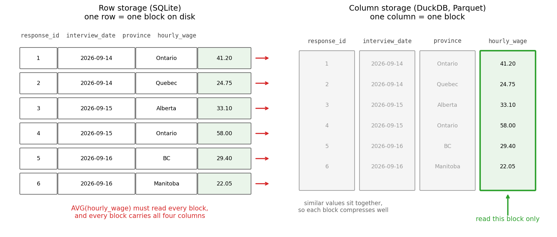
The column storage we can test this claim on is DuckDB: like SQLite it is free, runs inside the notebook, and keeps its data in a single file or in memory, and unlike SQLite it stores columns and processes them in bulk. It has one more trick which is amazing for our use case: it can see the dataframes in your session and query them by name. We don’t have to re-run everything. The .df() on the end of a DuckDB command asks for the result as a dataframe, the job pd.read_sql has been doing for SQLite:
duck = duckdb.connect()
duck.execute("CREATE TABLE responses AS SELECT * FROM big")
duck.execute("SELECT COUNT(*) AS loaded FROM responses").df()| loaded | |
|---|---|
| 0 | 250000 |
Now the identical question:
start = time.perf_counter()
duck_answer = duck.execute(question).df()
print(f"DuckDB: {1000 * (time.perf_counter() - start):.0f} ms")
duck_answer
DuckDB: 13 ms| province | responses | avg_wage | |
|---|---|---|---|
| 0 | Manitoba | 9831 | 38.95 |
| 1 | Ontario | 105559 | 38.74 |
| 2 | Alberta | 32430 | 38.69 |
| 3 | Saskatchewan | 7499 | 38.68 |
| 4 | British Columbia | 37095 | 38.66 |
| 5 | Quebec | 57586 | 38.60 |
Identical command on an identical table, and on this machine tens of times faster, down to single-digit milliseconds. Notebook 1 said SQL is declarative: you state what you want and the engine decides how. This is proof of that. We gave the same command to two different engines, and they chose differently because their storage shapes differ, one reading every block of every row, the other reading two column strips.
Neither engine is the better one. SQLite wins the intake workload of many small precious writes, DuckDB wins the analytical workload of few enormous reads, and the same organization usually needs both at once. This core tension, and the industry’s solution to it, is the whole of Notebook 7.
8. What format to keep it in
The last question is the archive. The office will keep the raw response history for years, outside any database, in files. The most obvious answer is CSV, which is where we started this stream. Let us give the intuitive answer a fair test:
start = time.perf_counter()
big.to_csv("datasets/wage_responses.csv", index=False)
print(f"CSV: written in {time.perf_counter() - start:.1f} s, "
      f"{os.path.getsize('datasets/wage_responses.csv') / 1e6:.0f} MB")
CSV: written in 0.7 s, 15 MBPredict first. The same dataframe is about to be written as Parquet, a format designed for exactly this job. It stores columns rather than rows, section 7’s idea carried into the file itself, and compresses each column strip. The CSV is about 15 MB. What about the Parquet?
start = time.perf_counter()
big.to_parquet("datasets/wage_responses.parquet")
print(f"Parquet: written in {time.perf_counter() - start:.1f} s, "
      f"{os.path.getsize('datasets/wage_responses.parquet') / 1e6:.0f} MB")
Parquet: written in 0.2 s, 3 MB3 MB, five times smaller, written faster than the CSV. (to_parquet works because the pyarrow library is installed; it is the standard engine for Parquet in Python.) Reading shows the same order:
start = time.perf_counter()
from_csv = pd.read_csv("datasets/wage_responses.csv")
print(f"read the CSV back:     {time.perf_counter() - start:.2f} s")

start = time.perf_counter()
from_parquet = pd.read_parquet("datasets/wage_responses.parquet")
print(f"read the Parquet back: {time.perf_counter() - start:.2f} s")
read the CSV back: 0.17 s
read the Parquet back: 0.13 sAn insignificant gap at this size can balloon at real scale, where a CSV must be parsed character by character while Parquet’s columns load nearly ready to use. But speed and size are a far smaller reason to choose Parquet compared to the next part. Compare what survived the round trip:
print("interview_date from the CSV:    ", from_csv["interview_date"].dtype)
print("interview_date from the Parquet:", from_parquet["interview_date"].dtype)
interview_date from the CSV: object
interview_date from the Parquet: datetime64[ns]The CSV returned our dates as object, which is plain text, because a CSV stores no types at all, and every read_csv starts the guessing game that opened Notebook 4. The Parquet returned datetime64, exactly what we wrote, because a Parquet file carries a schema inside it: every column’s name and type travel with the data. Notebook 5 taught that types belong in the schema, and Parquet is that idea for files. An archive that cannot forget its own types is an archive Notebook 4 never has to rescue.
One more payoff, DuckDB treats a Parquet file as a table you can query in place, no loading step at all:
duck.execute("""SELECT province, ROUND(AVG(hourly_wage), 2) AS avg_wage
                FROM 'datasets/wage_responses.parquet'
                GROUP BY province
                ORDER BY avg_wage DESC
LIMIT 3""").df()| province | avg_wage | |
|---|---|---|
| 0 | Manitoba | 38.95 |
| 1 | Ontario | 38.74 |
| 2 | Alberta | 38.69 |
That is a query running against a file sitting in a folder. A pile of Parquet files sitting in some cheap storage plus an engine that queries them is what industry calls a data lake, and we will talk about it more in Notebook 7.
9. Conclusion
The launch review gets its three answers, each with an experiment attached, and we can go home early. A crash mid-write cannot half-save an interview: transactions are atomic, the batch that died with the laptop left zero rows, and a second connection stayed isolated from uncommitted work. Respondent lookup stays instant at scale: an index took the search from a scan of everything to a tree walk, EXPLAIN QUERY PLAN proved the strategy changed, and the cost was a sixth more disk and slower writes. And the archive goes to Parquet, smaller than CSV, faster, and carrying its schema inside, with DuckDB querying it in place for the research archive.
Underneath all three runs one idea: the shape data takes on disk decides what is fast, what is safe, and what is possible. The intake side wants rows, transactions, and an index on respondents. The research side wants columns and doesn’t care about single rows. One copy of the data cannot be the best shape for both jobs, and pretending otherwise is where a lot of slow systems come from. Splitting the two properly is Notebook 7.
You can now answer these interview questions
- What is a transaction, and what does ACID stand for?
- A production query is slow. How do you diagnose it, how do you fix it, and what does the fix cost?
- Why do analytical databases store data by column?
- Why would you archive data as Parquet instead of CSV?
Show / hide model answers
- A group of statements the database applies as one unit. Atomic: all or nothing. Consistent: every rule holds before and after. Isolated: concurrent connections do not see each other’s unfinished work. Durable: once committed, a crash loses nothing.
- Read its plan with
EXPLAIN QUERY PLAN(orEXPLAINelsewhere); aSCANon a large table with a selective filter wants an index on the filtered column, turning the scan into aSEARCH. The cost is disk space and slower writes, since every insert or update must also maintain the index. - Analytical queries touch few columns of many rows. Storing each column together means reading only the columns the query names, and similar neighbouring values compress well, so the engine moves far fewer bytes for the same answer.
- Parquet is column-oriented and compressed, several times smaller and faster to read than CSV, and it stores each column’s type inside the file, so nothing about the data has to be guessed on the way back in.
Connections
- Back to Notebook 5: the schema said what may be stored; this notebook was how it is stored. The all-or-nothing behaviour behind Notebook 5’s refused load now has its name and its mechanism, the atomic transaction.
- Forward to Notebook 7: we saw one engine win at writing rows and another at reading columns. Next, the architecture built on that split: transactional and analytical databases, star schemas, the ETL between them, and where warehouses and lakes fit.
References
- Haerder, T., & Reuter, A. (1983). Principles of transaction-oriented database recovery. ACM Computing Surveys, 15(4), 287-317. The paper that coined ACID.
- Kleppmann, M. (2017). Designing Data-Intensive Applications. O’Reilly. Chapter 3 is this notebook in book form: B-trees, column storage, and why each exists.
- Malan, D. (2024). CS50’s Introduction to Databases with SQL. Harvard University. https://cs50.harvard.edu/sql/ The lecture on optimizing covers indexes and transactions.
- SQLite. Atomic commit in SQLite. https://www.sqlite.org/atomiccommit.html How the journal file makes section 4’s crash survivable.
- SQLite. EXPLAIN QUERY PLAN. https://www.sqlite.org/eqp.html Reading SCAN and SEARCH, from the engine’s own documentation.
- Winand, M. Use the Index, Luke! https://use-the-index-luke.com A free book on indexes and the queries that use or defeat them.
- DuckDB. Why DuckDB. https://duckdb.org/why_duckdb The design goals behind section 7’s benchmark.
- Apache Software Foundation. Apache Parquet documentation. https://parquet.apache.org/docs/ The column format carrying section 8’s schema.