Show the code
# Uncomment the line below to install packages:
#!pip install pytesseract easyocr opencv-python Pillow matplotlib pandas numpy nltk jiwer pdf2image "surya-ocr>=0.9" poppler anthropicBefore we begin, we need to install and import the necessary libraries. This notebook uses several Python packages for OCR, image processing, and text analysis.
Installation Note: If you’re running this notebook for the first time, uncomment and run the installation commands below. Some libraries require additional system dependencies:
conda install poppler or system package managerInstall the necessary packages:
# Uncomment the line below to install packages:
#!pip install pytesseract easyocr opencv-python Pillow matplotlib pandas numpy nltk jiwer pdf2image "surya-ocr>=0.9" poppler anthropicLoad the required packages:
import os
import re
os.environ["KMP_DUPLICATE_LIB_OK"] = "TRUE" # avoid OpenMP conflicts between libraries
import json
import warnings
warnings.filterwarnings('ignore')
import copy
from PIL import Image, ImageDraw, ImageFont
import cv2
import numpy as np
import easyocr
import pandas as pd
import matplotlib.pyplot as plt
import nltk
from nltk.tokenize import word_tokenize, sent_tokenize
from nltk.stem import PorterStemmer, WordNetLemmatizer
from jiwer import wer, cer
from pdf2image import convert_from_path
import gc
import torch
from surya.foundation import FoundationPredictor
from surya.recognition import RecognitionPredictor
from surya.detection import DetectionPredictor
from surya.layout import LayoutPredictor
from surya.settings import settings
nltk.download('punkt')
nltk.download('wordnet')
[nltk_data] Downloading package punkt to
[nltk_data] C:\Users\alexr\AppData\Roaming\nltk_data...
[nltk_data] Package punkt is already up-to-date!
[nltk_data] Downloading package wordnet to
[nltk_data] C:\Users\alexr\AppData\Roaming\nltk_data...
[nltk_data] Package wordnet is already up-to-date!TrueHere we define helper functions for loading and displaying images, and prepare the output directory. These functions will help us a lot throughout the notebook.
def load_image(path):
    #Load an image from pdf, jp2, tif, jpg, or png and return as RGB numpy array.
    if path.endswith('.pdf'):
        from pdf2image import convert_from_path
        pages = convert_from_path(path, dpi=300)
        return np.array(pages[0])
    else:
        img = Image.open(path)
        if img.mode != 'RGB':
            img = img.convert('RGB')
        return np.array(img)

def display_image(img, title="Image", figsize=(10, 8)):
    plt.figure(figsize=figsize)
    if len(img.shape) == 2:
        plt.imshow(img, cmap='gray')
    else:
        plt.imshow(img)
    plt.title(title)
    plt.axis('off')
    plt.tight_layout()
    plt.show()
    plt.close()

def display_images_side_by_side(img1, img2, title1="Before", title2="After", figsize=(14, 6)):
    fig, axes = plt.subplots(1, 2, figsize=figsize)

    if len(img1.shape) == 2:
        axes[0].imshow(img1, cmap='gray')
    else:
        axes[0].imshow(img1)
    axes[0].set_title(title1)
    axes[0].axis('off')

    if len(img2.shape) == 2:
        axes[1].imshow(img2, cmap='gray')
    else:
        axes[1].imshow(img2)
    axes[1].set_title(title2)
    axes[1].axis('off')

    plt.tight_layout()
    plt.show()
    plt.close()

os.makedirs('output', exist_ok=True)
print("Output directory ready: ./output/")
Output directory ready: ./output/Before we begin it is important to define how a computer can read text in the first place.
Humans and computers see text, and images differently. When you open a scanned document or a photograph of a page on your computer, you can read the words on screen but your computer cannot. You can see the context and what the image or text represents, but from a computer’s perspective there is no difference from a photograph of a landscape. In this case images are treated as visual, pixel-based graphics which are rendered onto your computer monitor, but the computer does not know exactly what it is rendering the same way a human viewing the images does. It could be a picture of your family, the ocean, a letter or a painting.
Machine-readable text, by contrast, is stored as character data (e.g., Unicode, or ASCII ) that software can search, sort, count, and analyze. A PDF or a Word document already contains machine-readable text. A normal picture does not. This distinction matters because nearly every computational text-analysis method (keyword search, topic modeling, named-entity recognition, embeddings) requires machine-readable text as input. If your source material exists only as images (scans, photographs, microfilm captures), you need a way to bridge the gap. That is exactly what OCR does.
Optical Character Recognition (OCR) is the technology that converts different types of documents: scanned paper documents, photographs of text, or images containing text into editable and searchable digital text.
For humanities researchers, OCR makes it possible to work with historical documents at scale, enabling:
By the end of this notebook, you will be able to:
Text extraction from documents falls into three main categories:
| Tool | Type | Strengths | Best For |
|---|---|---|---|
| Tesseract | Open-source | Fast, accurate on clean text | Printed documents |
| EasyOCR | Open-source | Multi-language, deep learning | Diverse scripts |
| Surya OCR | Open-source | Multi-language, layout detection, CPU-friendly | Complex layouts |
| Transkribus | Freemium | Excellent HTR, crowdsourcing | Handwritten documents |
| Azure Document Intelligence | Paid | Enterprise-grade, form extraction | Business documents |
| AWS Textract | Paid | Table extraction, scalable | Structured documents |
Traditional OCR systems convert images of text into machine-readable characters through a multi-stage pipeline. While early OCR relied on template matching (comparing characters against a library of known fonts), modern tools like EasyOCR and Tesseract use deep learning to achieve far greater accuracy.
Most OCR systems follow a two-stage process:
Text Detection: First, the system locates where text appears in the image. This involves identifying bounding boxes around words, lines, or paragraphs. Deep learning models scan the image and predict regions likely to contain text, even when text is rotated, curved, or partially obscured.
Text Recognition: Once text regions are detected, a separate model reads what the text says. This typically uses a neural network architecture called a CRNN (Convolutional Recurrent Neural Network) that processes the image sequence and outputs a string of characters. You can read more about CNNs at A Related Notebook.
Traditional template-matching OCR required near-perfect conditions: clean scans, standard fonts, and horizontal text. Deep learning models learn patterns from millions of examples, enabling them to:
EasyOCR specifically uses a CRAFT (Character Region Awareness for Text) detector for finding text, paired with a CRNN-based recognizer. This combination makes it particularly effective for documents with complex layouts or mixed content.
EasyOCR is a newer, deep-learning-based OCR library that supports 80+ languages. It provides built-in support for detecting text regions.
GPU Acceleration: EasyOCR can use GPU for faster processing. If you have a CUDA-capable GPU, it will be automatically detected. On CPU, processing may take a few seconds.
We will first load our sample image, a clean newspaper column:
img_path = "data/simple/newspaper_clean_col1.jp2"
img = load_image(img_path)
display_image(img, title="Sample Newspaper Column", figsize=(8, 12))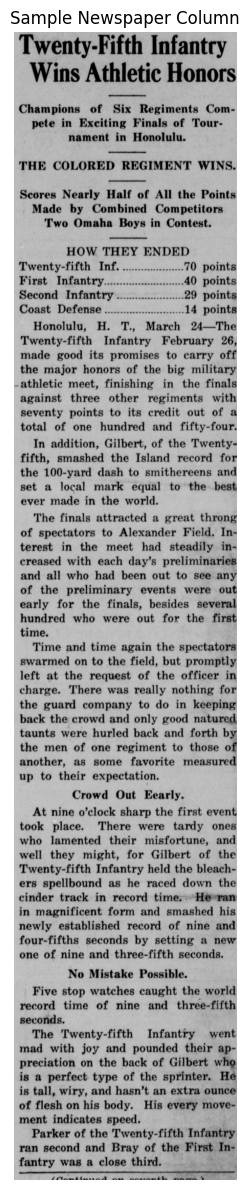
This is just one vertical column of clear text, for this notebook this will act as our most basic example.
We load the EasyOCR package and set it to read English with easyocr.Reader(['en']).
reader = easyocr.Reader(['en'], gpu=torch.cuda.is_available())Using CPU. Note: This module is much faster with a GPU.results = reader.readtext(img)
print(f"EasyOCR detected {len(results)} text regions")
print("\nFirst 10 detections:")
for i, (bbox, text, conf) in enumerate(results[:10]):
print(f" {i+1}. '{text}' (confidence: {conf:.2%})")
extracted_text = '\n'.join([text for (bbox, text, conf) in results])
ocr_df = pd.DataFrame({
'text': [text for (bbox, text, conf) in results],
'conf': [conf * 100 for (bbox, text, conf) in results]
})
print(f"\nTotal text length: {len(extracted_text)} characters")
print(f"Average confidence: {ocr_df['conf'].mean():.1f}%")EasyOCR detected 246 text regions
First 10 detections:
1. 'Twenty-Fifth Infantcy' (confidence: 62.46%)
2. 'Wins Athletic Honors' (confidence: 83.43%)
3. 'Champions' (confidence: 100.00%)
4. 'of' (confidence: 97.88%)
5. 'Six' (confidence: 99.99%)
6. 'Regiments' (confidence: 88.16%)
7. 'Com -' (confidence: 97.59%)
8. 'pete' (confidence: 99.44%)
9. 'in' (confidence: 99.98%)
10. 'Exciting Finals of' (confidence: 93.86%)
Total text length: 2348 characters
Average confidence: 91.4%EasyOCR scanned the newspaper image and identified 246 separate regions containing text, returning each one with its bounding box coordinates, the recognized text, and a confidence score.
Confidence scores are numerical metrics; typically ranging from 0 to 1 (0% to 100%) which indicates an AI or machine learning model’s level of certainty in its prediction or classification. They represent the probability that the model’s output is correct. A more technical definition is that: When an OCR model predicts a character, it computes a softmax probability distribution over all possible output classes. The confidence score is the maximum probability (the model’s estimated likelihood that its top prediction is correct). For example if an OCR model sees a deformed or smudged e it does not say immediately that it is an e, but calculates a probability for all characters (e,c,a,7,.,0 etc). The confidence score we see is the highest value of this prediction. This is a simplified description, the exact computation varies by model architecture (e.g. CTC-based models like EasyOCR compute sequence-level probabilities, while transformer models like Surya use token-level log-probabilities); but the intuition is the same: higher scores mean the model is more certain.
Crucially confidence scores are not accuracy, softmax normalizes over the model’s known vocabulary, not over ground truth. It is a valuable metric, but do not overly rely on it or tunnel vision on pushing the highest confidence. Low confidence is often more informative than high, it gives insights on the model’s true uncertainty.
One advantage of EasyOCR is that it provides polygonal bounding boxes that can better fit rotated or curved text:
img_with_boxes = img.copy()

for (bbox, text, conf) in results:
    pts = np.array(bbox, dtype=np.int32)
    color = (0, int(255 * conf), int(255 * (1 - conf))) # green=high, red=low
    cv2.polylines(img_with_boxes, [pts], isClosed=True, color=color, thickness=2)

display_image(img_with_boxes, title="EasyOCR Text Detections (Green=High Conf, Red=Low Conf)", figsize=(10, 14))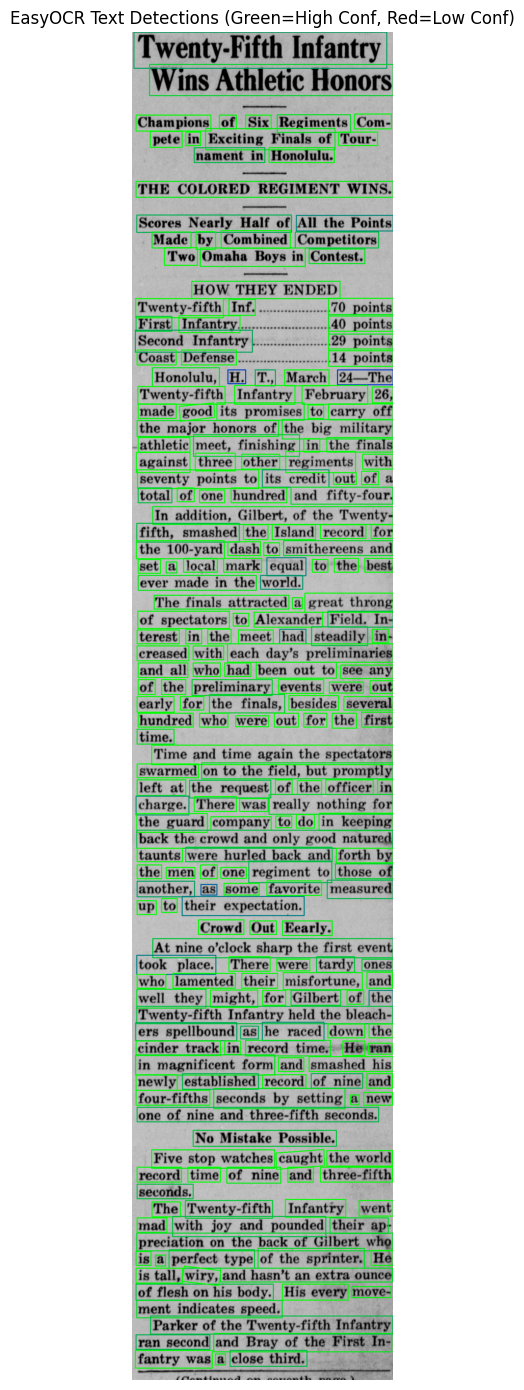
We can very clearly visually see the way in which EasyOCR is reading the text. Green boxes represent high confidence while red are lower confidence (we do not see any fully red boxes as there are no very low confidence regions).
The overall confidence from EasyOCR is at 91.4% which is not bad, but it is worth keeping in mind that this is a very basic example and the model is still making some mistakes. If we were to use a more difficult sample EasyOCR will struggle.
While open-source tools work well for many use cases, commercial solutions offer additional features:
| Tool | Pricing | Key Features | Best For |
|---|---|---|---|
| Transkribus | Freemium (~50 pages/month free via credit system) | HTR, crowdsourcing, model training | Historical manuscripts |
| Arkindex | Free for researchers | Document processing pipelines | Archives |
| eScriptorium | Free (self-hosted) | Medieval manuscripts, collaborative | Academic projects |
| Azure Document Intelligence | Basic OCR ~$1.50/1000 pages; forms/tables $10–$65/1000 | Form extraction, tables, structure | Business documents |
| AWS Textract | Basic OCR ~$1.50/1000 pages; structured extraction higher | Tables, forms, scalable API | Enterprise integration |
| Google Cloud Vision | Basic OCR ~$1.50/1000 images; Document AI higher | Multi-language, handwriting | Diverse content |
At the other end of the spectrum from traditional OCR are Vision Language Models (VLMs). These take a fundamentally different approach to document understanding. Rather than recognizing characters individually like traditional OCR, VLMs understand documents as a whole, interpreting text, layout, and visual context together.
| Approach | Traditional OCR | Vision Language Models |
|---|---|---|
| Method | Character-by-character recognition | Whole-document understanding |
| Layout | Separate step | Integrated |
| Context | Limited | Full document context |
| Errors | Isolated character mistakes | More coherent (or coherently wrong!) |
Use Traditional OCR when:
Use VLMs when:
GPU Requirements: Most VLMs require significant GPU memory (8GB+). For CPU-only systems, consider Surya OCR which works well on CPU.
Vision Language Models combine two powerful components: a vision encoder that “sees” the image and a language model that “reasons” about what it sees. This architecture allows them to understand documents the way humans do; taking in the whole page at once rather than reading character by character.
VLMs typically follow a three-stage process:
Visual Encoding: The image is divided into small patches (like tiles in a mosaic) and processed by a vision encoder. Often a Vision Transformer (ViT). This converts the raw pixels into a sequence of visual embeddings that capture shapes, patterns, and spatial relationships.
Cross-Modal Fusion: The visual embeddings are combined with text understanding capabilities. This can happen through:
Text Generation: A language model (often a transformer decoder) generates the output text, guided by what it “saw” in the image. Because this is a language model, it can produce grammatically coherent text and use context to fill in gaps.
Traditional OCR processes text in isolation; each character or word is recognized independently. VLMs take a fundamentally different approach, they have the whole context of the document and can generate correct grammatical sentences based on that context. They also have built-in layout understanding as they can “see” the document.
For example, if a historical document has a smudged word, traditional OCR might output nonsense characters. A VLM can use surrounding context like the topic of the paragraph, common phrases of the era, grammatical structure in order to infer the most likely word.
The Trade-off: VLMs are more powerful but also much more resource-intensive. They excel at understanding what a document means but may sometimes “hallucinate” plausible-sounding text that wasn’t actually in the image. This will be familiar to anyone who has used ChatGPT or other LLMs in the past. Traditional OCR is more literal. It only outputs what it detects, errors and all.
Full VLMs like GPT-4V or Gemini are powerful but require significant computational resources, often cloud-hosted GPUs and API costs. For this notebook we use Surya OCR instead, a practical middle ground. Surya is not a VLM in the strict sense, but it borrows ideas from that world: it uses transformer-based models and includes built-in layout analysis alongside text detection and recognition. It works well on CPU, supports 90+ languages, and does not require cloud access or API keys.
Let’s try running Surya OCR on the same newspaper column and look at the results. This will take longer to run than EasyOCR. We can then compare the confidence and findings.
foundation_predictor = FoundationPredictor()
rec_predictor = RecognitionPredictor(foundation_predictor)
det_predictor = DetectionPredictor()

surya_img = Image.fromarray(img)
surya_results = rec_predictor([surya_img], det_predictor=det_predictor)
surya_result = surya_results[0]

surya_texts = [line.text for line in surya_result.text_lines]
surya_scores = [line.confidence for line in surya_result.text_lines]

print(f"Surya OCR detected {len(surya_texts)} text regions")
print("\nFirst 10 detections:")
for i, (text, conf) in enumerate(zip(surya_texts[:10], surya_scores[:10])):
    print(f"  {i+1}. '{text}' (confidence: {conf:.2%})")

surya_full_text = ' '.join(surya_texts)
print(f"\n[Total characters extracted: {len(surya_full_text)}]")
print(f"Average confidence: {np.mean(surya_scores):.1%}")
print("\nFull text preview:")
print(surya_full_text[:2000])

del rec_predictor, det_predictor, foundation_predictor
gc.collect()
if torch.cuda.is_available():
    torch.cuda.empty_cache()
Detecting bboxes: 0%| | 0/1 [00:00<?, ?it/s]Detecting bboxes: 100%|██████████| 1/1 [00:23<00:00, 23.78s/it]Detecting bboxes: 100%|██████████| 1/1 [00:23<00:00, 23.84s/it]
Recognizing Text: 0%| | 0/73 [00:00<?, ?it/s]Recognizing Text: 1%|▏ | 1/73 [00:47<56:50, 47.37s/it]Recognizing Text: 3%|▎ | 2/73 [00:47<23:16, 19.67s/it]Recognizing Text: 4%|▍ | 3/73 [00:49<13:14, 11.35s/it]Recognizing Text: 5%|▌ | 4/73 [00:49<08:07, 7.06s/it]Recognizing Text: 8%|▊ | 6/73 [00:50<03:59, 3.57s/it]Recognizing Text: 10%|▉ | 7/73 [00:51<03:04, 2.79s/it]Recognizing Text: 19%|█▉ | 14/73 [00:55<01:10, 1.19s/it]Recognizing Text: 25%|██▍ | 18/73 [00:55<00:42, 1.30it/s]Recognizing Text: 32%|███▏ | 23/73 [00:58<00:34, 1.44it/s]Recognizing Text: 41%|████ | 30/73 [01:02<00:25, 1.67it/s]Recognizing Text: 44%|████▍ | 32/73 [01:02<00:22, 1.84it/s]Recognizing Text: 45%|████▌ | 33/73 [01:10<00:49, 1.25s/it]Recognizing Text: 47%|████▋ | 34/73 [01:10<00:43, 1.12s/it]Recognizing Text: 51%|█████ | 37/73 [01:12<00:36, 1.00s/it]Recognizing Text: 52%|█████▏ | 38/73 [01:13<00:32, 1.07it/s]Recognizing Text: 55%|█████▍ | 40/73 [01:13<00:23, 1.43it/s]Recognizing Text: 60%|██████ | 44/73 [01:15<00:16, 1.80it/s]Recognizing Text: 68%|██████▊ | 50/73 [01:15<00:06, 3.31it/s]Recognizing Text: 75%|███████▌ | 55/73 [01:15<00:03, 4.80it/s]Recognizing Text: 81%|████████ | 59/73 [01:15<00:02, 6.09it/s]Recognizing Text: 84%|████████▎ | 61/73 [01:16<00:01, 6.36it/s]Recognizing Text: 86%|████████▋ | 63/73 [01:17<00:02, 4.01it/s]Recognizing Text: 88%|████████▊ | 64/73 [01:17<00:02, 3.58it/s]Recognizing Text: 89%|████████▉ | 65/73 [01:18<00:03, 2.61it/s]Recognizing Text: 90%|█████████ | 66/73 [01:18<00:02, 2.78it/s]Recognizing Text: 92%|█████████▏| 67/73 [01:19<00:02, 2.58it/s]Recognizing Text: 95%|█████████▍| 69/73 [01:19<00:01, 3.00it/s]Recognizing Text: 96%|█████████▌| 70/73 [01:20<00:00, 3.18it/s]Recognizing Text: 99%|█████████▊| 72/73 [01:20<00:00, 4.08it/s]Recognizing Text: 100%|██████████| 73/73 [01:20<00:00, 4.08it/s]Recognizing Text: 100%|██████████| 73/73 [01:20<00:00, 1.11s/it]Surya OCR detected 73 text regions
First 10 detections:
1. '<b>Twenty-Fifth Infantry</b>' (confidence: 98.09%)
2. '<b>Wins Athletic Honors</b>' (confidence: 97.80%)
3. 'Champions of Six Regiments Com-' (confidence: 99.36%)
4. 'pete in Exciting Finals of Tour-' (confidence: 99.68%)
5. 'nament in Honolulu.' (confidence: 99.78%)
6. 'THE COLORED REGIMENT WINS.' (confidence: 99.84%)
7. 'Scores Nearly Half of All the Points' (confidence: 99.43%)
8. 'Made by Combined Competitors' (confidence: 98.73%)
9. 'Two Omaha Boys in Contest.' (confidence: 99.55%)
10. 'HOW THEY ENDED' (confidence: 98.47%)
[Total characters extracted: 2384]
Average confidence: 99.4%
Full text preview:
<b>Twenty-Fifth Infantry</b> <b>Wins Athletic Honors</b> Champions of Six Regiments Com- pete in Exciting Finals of Tour- nament in Honolulu. THE COLORED REGIMENT WINS. Scores Nearly Half of All the Points Made by Combined Competitors Two Omaha Boys in Contest. HOW THEY ENDED Twenty-fifth Inf. .....70 points First Infantry.....40 points Second Infantry ......29 points Coast Defense .....14 points Honolulu, H. T., March 24-The Twenty-fifth Infantry February 26, made good its promises to carry off the major honors of the big military athletic meet, finishing in the finals against three other regiments with seventy points to its credit out of a total of one hundred and fifty-four. In addition, Gilbert, of the Twenty- fifth, smashed the Island record for the 100-yard dash to smithereens and set a local mark equal to the best ever made in the world. The finals attracted a great throng of spectators to Alexander Field. In- terest in the meet had steadily in- creased with each day's preliminaries and all who had been out to see any of the preliminary events were out early for the finals, besides several hundred who were out for the first time. Time and time again the spectators swarmed on to the field, but promptly left at the request of the officer in charge. There was really nothing for the guard company to do in keeping back the crowd and only good natured taunts were hurled back and forth by the men of one regiment to those of another, as some favorite measured up to their expectation. Crowd Out Eearly. At nine o'clock sharp the first event took place. There were tardy ones who lamented their misfortune, and well they might, for Gilbert of the Twenty-fifth Infantry held the bleach- ers spellbound as he raced down the cinder track in record time. He ran in magnificent form and smashed his newly established record of nine and four-fifths seconds by setting a new one of nine and three-fifth seconds. No Mistake Possible. Five stop watches caught the world record time of niOutput text sample: “Twenty-Fifth Infantry Wins Athletic Honors Champions of Six Regiments Com- pete in Exciting Finals of Tour- nament in Honolulu. THE COLORED REGIMENT WINS. Scores Nearly Half of All the Points Made by Combined Competitors Two Omaha Boys in Contest.”
EasyOCR had an Average confidence: 91.4% while Surya had an average confidence of 99.4%. It is worth noting that confidence is not everything and it is important to actually review the results or compare them to a “ground-truth” (the actual text inside of the document often in a .txt format). The text preview looks correct, but this was a very simple example. Let’s try on something far more difficult.
Our example here will be a handwritten letter from the American Civil war from Alexander Parker Crittenden to his wife, Clara Crittenden dated to December 11, 1864. We can see how EasyOCR and Surya handle this more difficult handwritten example.
letter_pages = convert_from_path("data/simple/handwritten_letter_page1.pdf", dpi=300)
letter_img = np.array(letter_pages[0])
display_image(letter_img, title="Handwritten Letter (Civil War Era)", figsize=(10, 12))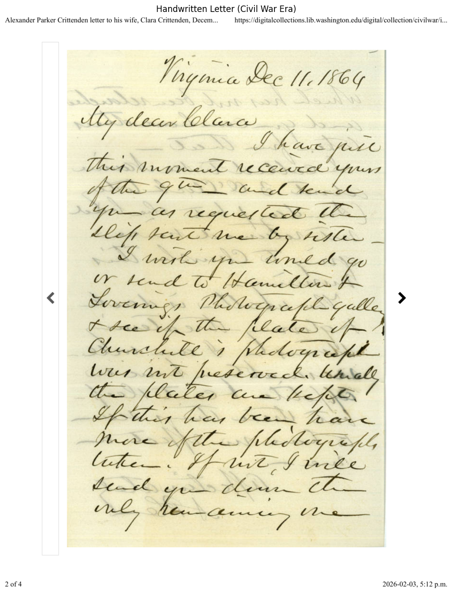
The text is handwritten in cursive along with there being lots of background noise from the next page bleeding into the frame. Let’s first try EasyOCR.
easyocr_hw_results = reader.readtext(letter_img)
easyocr_hw_text = '\n'.join([text for (bbox, text, conf) in easyocr_hw_results])
easyocr_hw_confs = [conf for (bbox, text, conf) in easyocr_hw_results]

print("EasyOCR:")
print(f"Regions detected: {len(easyocr_hw_results)}")
print(f"Avg confidence: {np.mean(easyocr_hw_confs):.2%}")
print(f"\nExtracted text (first 500 chars):\n{easyocr_hw_text[:500]}")
EasyOCR:
Regions detected: 61
Avg confidence: 29.82%
Extracted text (first 500 chars):
Alexander Parker Crittenden letter to his wife, Clara Crittenden; Decem.
https://digitalcollections lib.washington edu/digital/collection/civilwarli.
{ {
88>
5>
decv lelavc
3
Tlei aninezc
LCexucc Yuv
9
Cfc
Ic '
L
~ecue{EC
lcZ Alz_
1&
lu l
UinCc
U
[&xuaUz
Kv
Soscuzu
PLles ~[czadl
7 &i_
U
Rabs
4
ClusukU
luus
l
Acc
liual
hlaZez
Gheha
Y& ,
Ui
ha< <
Ia<
Uck _
EzZ
J
Lafc
2Z _
Ukl
Z
Laid
UlR~
2 of 4
2026-02-03, 5.12 p.m
'fnyuut
@ee
[S6 G
[
uf
kavc
(
kg
C1
btC Z
SA
~fzEasyOCR has performed very poorly and the output for the actual body of the letter is mostly random symbols and nonsensical. This is an excellent example to not follow average confidence blindly as the average confidence is 29.82% which should imply that it is slightly legible. The average confidence here is skewed by the lines above the letter from the University of Washington which are not handwritten.
Let’s try now with Surya:
foundation_predictor = FoundationPredictor()
rec_predictor_hw = RecognitionPredictor(foundation_predictor)
det_predictor_hw = DetectionPredictor()

surya_hw_img = Image.fromarray(letter_img)
surya_hw_results = rec_predictor_hw([surya_hw_img], det_predictor=det_predictor_hw)
surya_hw_result = surya_hw_results[0]

surya_hw_texts = [line.text for line in surya_hw_result.text_lines]
surya_hw_scores = [line.confidence for line in surya_hw_result.text_lines]
surya_hw_text = '\n'.join(surya_hw_texts)

print("--- Surya OCR ---")
print(f"Regions detected: {len(surya_hw_texts)}")
print(f"Avg confidence: {np.mean(surya_hw_scores):.2%}")
print(f"\nExtracted text (first 500 chars):\n{surya_hw_text[:500]}")

del rec_predictor_hw, det_predictor_hw, foundation_predictor
gc.collect()
if torch.cuda.is_available():
    torch.cuda.empty_cache()
Detecting bboxes: 0%| | 0/1 [00:00<?, ?it/s]Detecting bboxes: 100%|██████████| 1/1 [00:07<00:00, 7.25s/it]Detecting bboxes: 100%|██████████| 1/1 [00:07<00:00, 7.25s/it]
Recognizing Text: 0%| | 0/22 [00:00<?, ?it/s]Recognizing Text: 5%|▍ | 1/22 [00:56<19:51, 56.75s/it]Recognizing Text: 9%|▉ | 2/22 [00:57<07:51, 23.60s/it]Recognizing Text: 14%|█▎ | 3/22 [00:58<04:13, 13.34s/it]Recognizing Text: 18%|█▊ | 4/22 [00:59<02:33, 8.52s/it]Recognizing Text: 27%|██▋ | 6/22 [01:00<01:10, 4.41s/it]Recognizing Text: 36%|███▋ | 8/22 [01:01<00:37, 2.68s/it]Recognizing Text: 55%|█████▍ | 12/22 [01:02<00:13, 1.30s/it]Recognizing Text: 68%|██████▊ | 15/22 [01:03<00:06, 1.02it/s]Recognizing Text: 77%|███████▋ | 17/22 [01:04<00:03, 1.29it/s]Recognizing Text: 82%|████████▏ | 18/22 [01:04<00:02, 1.41it/s]Recognizing Text: 86%|████████▋ | 19/22 [01:05<00:02, 1.34it/s]Recognizing Text: 95%|█████████▌| 21/22 [01:25<00:03, 3.87s/it]Recognizing Text: 100%|██████████| 22/22 [01:26<00:00, 3.43s/it]Recognizing Text: 100%|██████████| 22/22 [01:26<00:00, 3.94s/it]--- Surya OCR ---
Regions detected: 22
Avg confidence: 87.35%
Extracted text (first 500 chars):
Alexander Parker Crittenden letter to his wife, Clara Crittenden, Decem...
https://digitalcollections.lib.washington.edu/digital/collection/civilwar/i...
Ingmia Dec 11, 1864
My dear Clara
This imment received yours
requested the
Elefi tant me by tester -
I wish you would go
or send to Itamellow to
Forenings Pholograph galle
the of the place of
Churchite i Midograph
wer not preserved unally
the places are kept
If this has been have
more of the photographs
Tur I ince
When if
send you down the
onlyThis output is far far better, Surya has read the text quite accurately. It is night and day from EasyOCR, it is not perfect but you can determine the general content of the letter.
comparison = pd.DataFrame({
    'Metric': ['Regions detected', 'Avg confidence', 'Total characters'],
    'EasyOCR': [len(easyocr_hw_results), f"{np.mean(easyocr_hw_confs):.2%}", len(easyocr_hw_text)],
    'Surya OCR': [len(surya_hw_texts), f"{np.mean(surya_hw_scores):.2%}", len(surya_hw_text)]
})
display(comparison)

del reader
gc.collect()
if torch.cuda.is_available():
torch.cuda.empty_cache()| Metric | EasyOCR | Surya OCR | |
|---|---|---|---|
| 0 | Regions detected | 61 | 22 |
| 1 | Avg confidence | 29.82% | 87.35% |
| 2 | Total characters | 468 | 542 |
Both engines struggle a bit more with handwritten text. Traditional OCR is built for printed characters, so the low confidence scores and garbled output here are expected. Surya, with its transformer-based approach, performs much better. We have seen both great OCR and poor OCR, so what can we do to get the best results, how can we help the models. You can just throw different models at text and hope it works, but there are many tools and techniques which can be used to improve the OCR quality. In the next section we will look at developing a full pipeline to give the models a leg-up by giving them the best possible source and then post-processing techniques to analyze the output.
A complete OCR workflow involves three stages: pre-processing, text extraction, and post-processing. Each stage can significantly impact final accuracy.
Pre-processing transforms raw document images into formats optimized for OCR. Each technique below uses a different image to highlight what that step does best.
Converting to grayscale simplifies the image from three colour channels (RGB) down to one. By removing colour, it reduces noise and improves contrast between text and background. This also lowers file size which is critical for computation time and can be very impactful for batch-processing lots of documents. Here we use a colour photograph of the UBC campus:
ubc_img = load_image("data/pre_processing_example/ubc_preprocess.jpg")
ubc_gray = cv2.cvtColor(ubc_img, cv2.COLOR_RGB2GRAY)
display_images_side_by_side(ubc_img, ubc_gray, "Original (UBC)", "Grayscale (UBC)")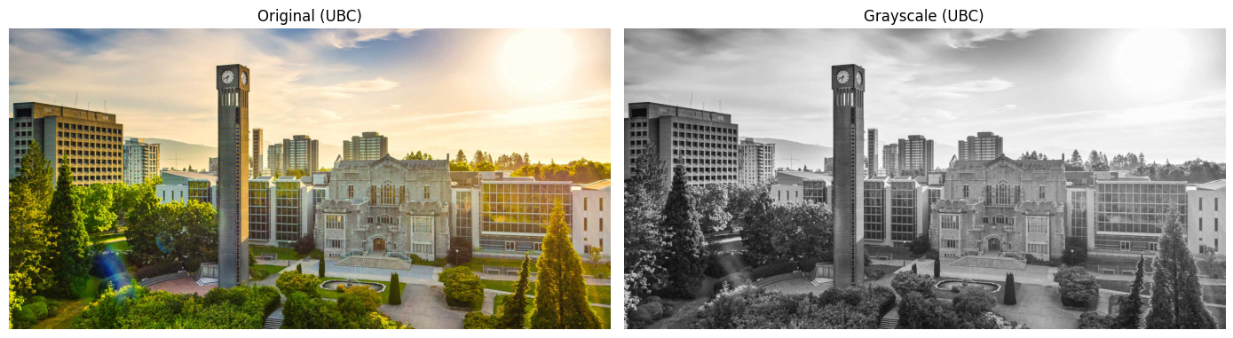
Now let’s try the same thing on a very different image — a handwritten restaurant menu on a blackboard:
menu_img = load_image("data/pre_processing_example/colourful-restaurant-menu-written-on-blackboard-style-sign-DH7FAJ.jpg")
menu_gray = cv2.cvtColor(menu_img, cv2.COLOR_RGB2GRAY)
display_images_side_by_side(menu_img, menu_gray, "Original (Menu)", "Grayscale (Menu)")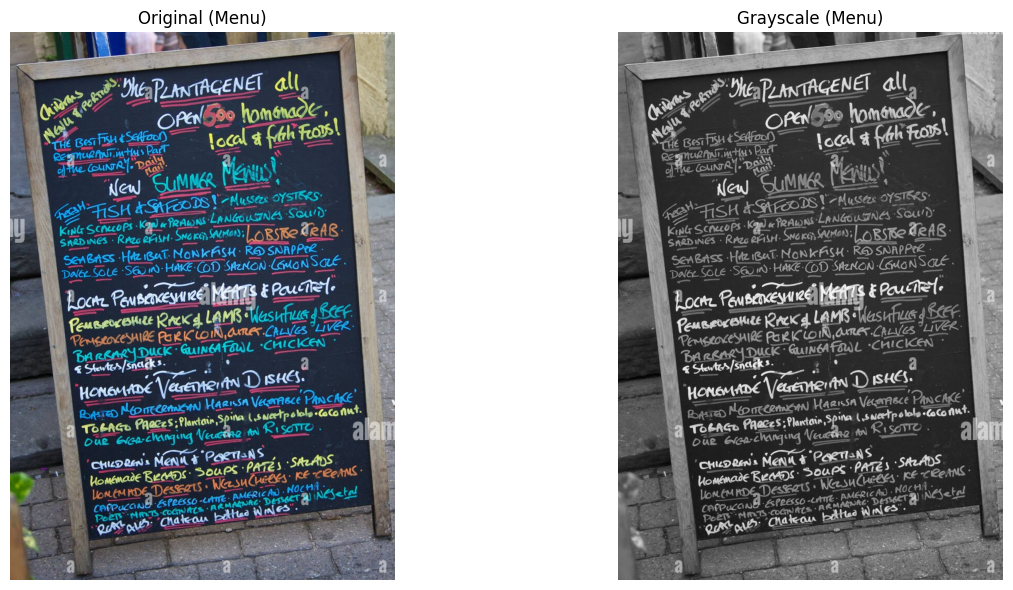
This will help OCR models “see” the text and extract it. Grayscale helps OCR clearly see and analyze text as it reduces color noise and channel complexity. The image is simplified and allows the model to extract the text.
Binarization converts the image to pure black and white. Otsu’s method is a global automatic image thresholding algorithm that converts grayscale images into binary (black and white) by determining an optimal threshold that separates pixels into foreground and background classes. It automatically finds the optimal threshold:
First we will apply Otsu’s method to our image of UBC to show what it does:
otsu_thresh, ubc_binary = cv2.threshold(ubc_gray, 0, 255, cv2.THRESH_BINARY + cv2.THRESH_OTSU)

print(f"Otsu selected threshold: {otsu_thresh:.0f} (out of 255)")
display_images_side_by_side(ubc_img, ubc_binary, "Original", "Otsu's Binarization")
Otsu selected threshold: 145 (out of 255)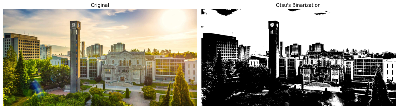
Now let’s apply binarization to a noisy newspaper page:
noisy_img = load_image("data/simple/newspaper_noisy.jp2")
noisy_gray = cv2.cvtColor(noisy_img, cv2.COLOR_RGB2GRAY)

otsu_thresh, otsu_binary = cv2.threshold(noisy_gray, 0, 255, cv2.THRESH_BINARY + cv2.THRESH_OTSU)

display_images_side_by_side(noisy_img, otsu_binary, "Original", "Otsu's Binarization")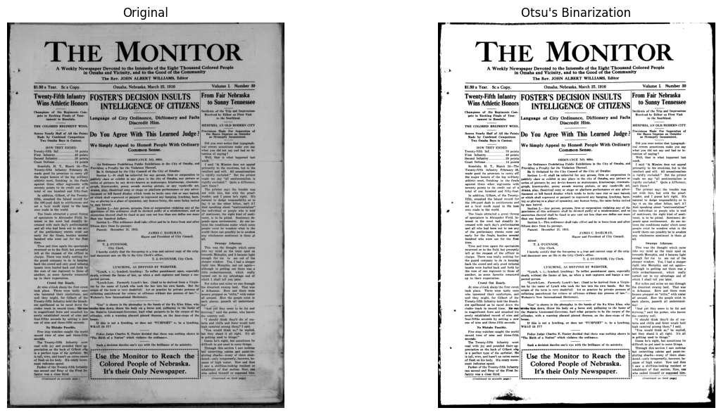
We can see that the end result is much clearer. It is black text on a pure white background as opposed to the gray, the smudges have also decreased on the margins of the newspaper.
Noise in images is “the random, unwanted variation in brightness or colour information in digital images, appearing as a grainy, speckled, or mottled texture.” An example is 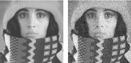
Removing noise can dramatically improve OCR accuracy. Let’s first see what denoising does on a noisy image without text:
noisy_notext = load_image("data/pre_processing_example/noise_cleanup_example_notext.png")
noisy_notext_gray = cv2.cvtColor(noisy_notext, cv2.COLOR_RGB2GRAY)

denoised_notext = cv2.fastNlMeansDenoising(noisy_notext_gray, h=10)
display_images_side_by_side(noisy_notext, denoised_notext, "Original (Noisy)", "Denoised")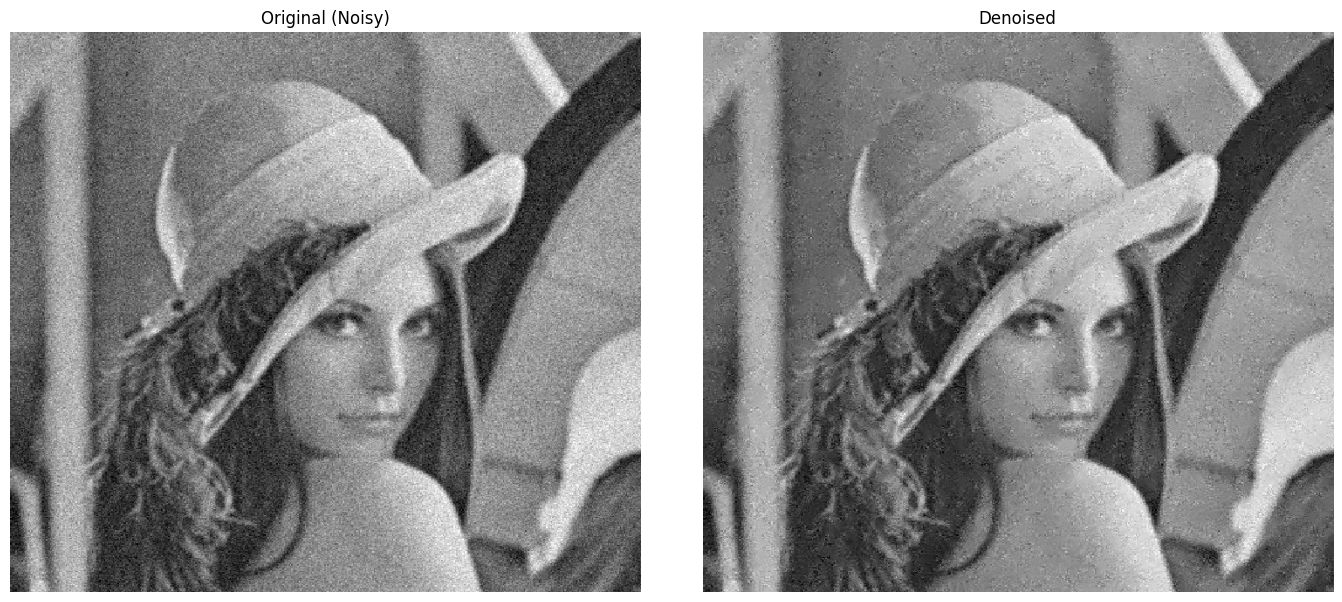
The image of the woman on the left has small visible specks on it which could hinder OCR quality, on the right it is far clearer.
Now let’s apply the same technique to a noisy image that contains text:
noisy_text = load_image("data/pre_processing_example/noise_text.png")
noisy_text_gray = cv2.cvtColor(noisy_text, cv2.COLOR_RGB2GRAY)

denoised_text = cv2.fastNlMeansDenoising(noisy_text_gray, h=10)
display_images_side_by_side(noisy_text, denoised_text, "Original (Noisy Text)", "Denoised")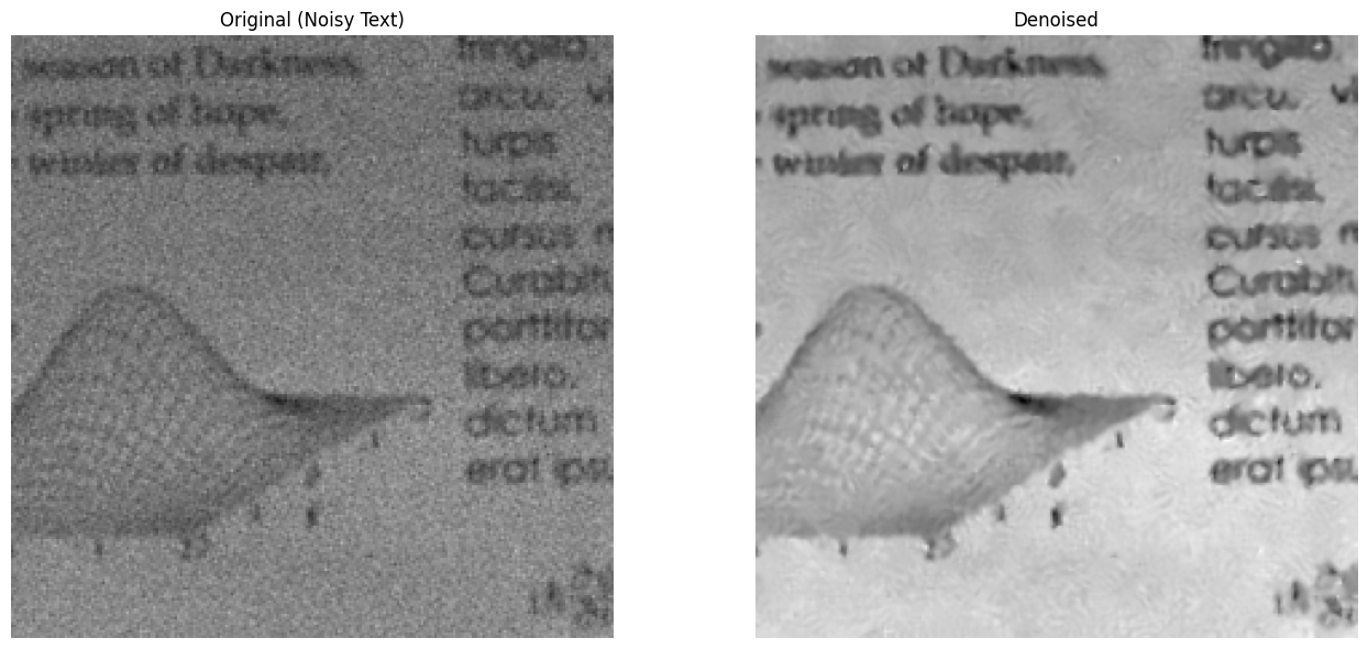
The text is much clearer and easier to read.
Rotated documents hurt OCR accuracy. Let’s detect and correct rotation:
First we will make a function called deskew which we will apply later in the notebook. It determines the skew of the image and then rotates it to be facing upwards.
# Detect skew angle via Hough lines and rotate to correct it
def deskew(image):
    if len(image.shape) == 3:
        gray = cv2.cvtColor(image, cv2.COLOR_RGB2GRAY)
    else:
        gray = image.copy()

    edges = cv2.Canny(gray, 50, 150, apertureSize=3)
    lines = cv2.HoughLines(edges, 1, np.pi/180, 200)

    if lines is None:
        return image, 0

    angles = []
    for rho, theta in lines[:, 0]:
        angle = np.degrees(theta) - 90
        if -45 < angle < 45:
            angles.append(angle)

    if not angles:
        return image, 0

    median_angle = np.median(angles)

    (h, w) = image.shape[:2]
    center = (w // 2, h // 2)
    M = cv2.getRotationMatrix2D(center, median_angle, 1.0)
    rotated = cv2.warpAffine(image, M, (w, h), flags=cv2.INTER_CUBIC,
                              borderMode=cv2.BORDER_REPLICATE)

    return rotated, median_angle
We now apply our deskew function on some example text:
skewed_img = load_image("data/pre_processing_example/deskew_example.jpg")
deskewed, angle = deskew(skewed_img)
print(f"Detected skew angle: {angle:.2f} degrees")

display_images_side_by_side(skewed_img, deskewed, "Original", f"Deskewed ({angle:.2f}°)")
Detected skew angle: -20.00 degrees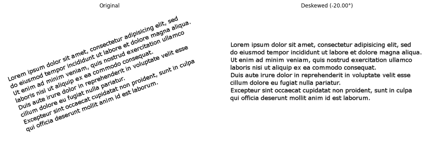
The text was dynamically rotated. This greatly improves OCR as skewed text hurts OCR accuracy because models expect horizontal baselines, even a few degrees of tilt causes character errors.
CLAHE (Contrast Limited Adaptive Histogram Equalization) improves readability of an image by fixing the lighting.
We will use our grayscale image of UBC and improve the contrast. CLAHE divides the image into small tiles and runs histogram equalization independently on each one, stretching brightness levels so the darks get darker and the lights get lighter. A contrast limit prevents over-amplification of noise in uniform regions.
clahe = cv2.createCLAHE(clipLimit=2.0, tileGridSize=(8, 8))
ubc_enhanced = clahe.apply(ubc_gray)

display_images_side_by_side(ubc_gray, ubc_enhanced, "Original Grayscale", "CLAHE Enhanced")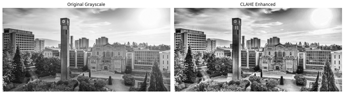
Over pre-processing: Doing too much pre-processing can degrade the image quality and make it nearly illegible. A clean PDF run through aggressive binarization + denoising will lose information. Be careful when running pre-processing, not every document needs every step. They can hurt more than help. Look at the output and test various techniques.
Historical newspapers and various other documents often have complex multi-column layouts. Without proper layout analysis, OCR might read across columns incorrectly.
Consider this scenario:
Column 1           Column 2
-----------        -----------
The mayor          Meanwhile,
announced today    across town
that the city      residents
Without layout analysis, OCR might read: “The mayor Meanwhile, announced today across town…”
Surya OCR includes a LayoutPredictor that detects and classifies document regions into types like Text, Table, Figure, SectionHeader, and more. It also assigns a reading order so you know which region to process first.
Let’s load our more difficult newspaper example and run Layout Analysis on it.
multicolumn_path = "data/simple/newspaper_multicolumn.jp2"
multicolumn_img = load_image(multicolumn_path)
multicolumn_pil = Image.fromarray(multicolumn_img)

display_image(multicolumn_img, title="Multi-Column Newspaper Front Page", figsize=(12, 14))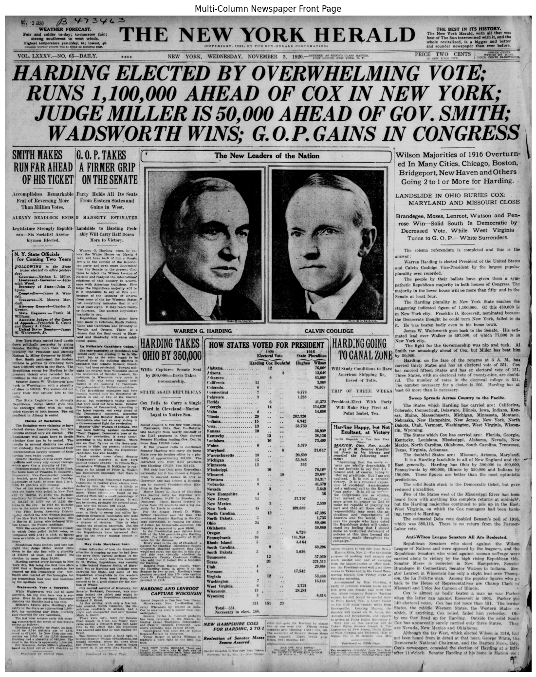
Compared to our single column, this is far more difficult with various columns, titles, images and sub-headings. We will run the Surya OCR LayoutPredictor which will detect regions of text and just like the EasyOCR example from earlier put boxes around them. It also comes with confidence scores.
foundation_predictor = FoundationPredictor(checkpoint=settings.LAYOUT_MODEL_CHECKPOINT)
layout_predictor = LayoutPredictor(foundation_predictor)

layout_results = layout_predictor([multicolumn_pil])
layout = layout_results[0]

print(f"Detected {len(layout.bboxes)} layout regions:\n")
for box in layout.bboxes:
    print(f"  [{box.label}] position {box.position}, confidence {box.confidence:.2%}")

del layout_predictor, foundation_predictor
gc.collect()
if torch.cuda.is_available():
    torch.cuda.empty_cache()
Recognizing Layout: 0%| | 0/1 [00:00<?, ?it/s]Recognizing Layout: 100%|██████████| 1/1 [00:26<00:00, 26.34s/it]Recognizing Layout: 100%|██████████| 1/1 [00:26<00:00, 26.34s/it]Detected 113 layout regions:
[PageHeader] position 0, confidence 76.75%
[PageHeader] position 1, confidence 57.76%
[PageHeader] position 2, confidence 86.22%
[Text] position 3, confidence 75.94%
[Text] position 4, confidence 80.20%
[Text] position 5, confidence 88.44%
[Text] position 6, confidence 97.85%
[Text] position 7, confidence 96.38%
[Text] position 8, confidence 96.42%
[SectionHeader] position 9, confidence 71.03%
[SectionHeader] position 10, confidence 71.15%
[Text] position 11, confidence 82.41%
[Text] position 12, confidence 97.44%
[Text] position 13, confidence 99.03%
[Text] position 14, confidence 60.36%
[Text] position 15, confidence 98.26%
[Text] position 16, confidence 97.85%
[Text] position 17, confidence 99.26%
[Text] position 18, confidence 99.52%
[Text] position 19, confidence 98.80%
[Text] position 20, confidence 99.93%
[Text] position 21, confidence 99.86%
[Text] position 22, confidence 99.86%
[SectionHeader] position 23, confidence 92.54%
[Text] position 24, confidence 99.94%
[Text] position 25, confidence 99.94%
[Text] position 26, confidence 99.96%
[Text] position 27, confidence 99.83%
[Text] position 28, confidence 99.85%
[Text] position 29, confidence 99.84%
[SectionHeader] position 30, confidence 70.92%
[Text] position 31, confidence 98.95%
[Text] position 32, confidence 99.69%
[Text] position 33, confidence 99.81%
[Text] position 34, confidence 91.56%
[Text] position 35, confidence 78.99%
[Text] position 36, confidence 95.13%
[Text] position 37, confidence 97.17%
[Text] position 38, confidence 97.77%
[Text] position 39, confidence 99.67%
[Text] position 40, confidence 99.75%
[Text] position 41, confidence 58.86%
[Text] position 42, confidence 96.98%
[Text] position 43, confidence 99.89%
[Text] position 44, confidence 99.97%
[Text] position 45, confidence 99.99%
[Text] position 46, confidence 99.91%
[SectionHeader] position 47, confidence 89.62%
[Text] position 48, confidence 99.97%
[Text] position 49, confidence 99.60%
[Text] position 50, confidence 99.80%
[Text] position 51, confidence 99.95%
[Text] position 52, confidence 99.94%
[Text] position 53, confidence 97.24%
[Text] position 54, confidence 52.97%
[Picture] position 55, confidence 96.68%
[Picture] position 56, confidence 74.31%
[Text] position 57, confidence 52.48%
[Text] position 58, confidence 88.91%
[SectionHeader] position 59, confidence 92.95%
[Text] position 60, confidence 95.98%
[Text] position 61, confidence 97.67%
[Text] position 62, confidence 99.42%
[Text] position 63, confidence 99.89%
[Text] position 64, confidence 99.99%
[Text] position 65, confidence 99.98%
[Text] position 66, confidence 99.96%
[Text] position 67, confidence 99.96%
[Text] position 68, confidence 99.74%
[Text] position 69, confidence 98.66%
[SectionHeader] position 70, confidence 98.18%
[Text] position 71, confidence 99.96%
[Text] position 72, confidence 99.97%
[Text] position 73, confidence 99.87%
[Text] position 74, confidence 91.55%
[SectionHeader] position 75, confidence 60.16%
[Table] position 76, confidence 90.22%
[Text] position 77, confidence 88.40%
[Text] position 78, confidence 98.59%
[Text] position 79, confidence 98.30%
[Text] position 80, confidence 98.73%
[SectionHeader] position 81, confidence 92.70%
[Text] position 82, confidence 99.64%
[Text] position 83, confidence 99.55%
[Text] position 84, confidence 99.83%
[SectionHeader] position 85, confidence 78.00%
[Text] position 86, confidence 99.89%
[Text] position 87, confidence 99.84%
[Text] position 88, confidence 99.34%
[Text] position 89, confidence 99.90%
[Text] position 90, confidence 98.18%
[Text] position 91, confidence 99.69%
[Text] position 92, confidence 97.21%
[Text] position 93, confidence 94.09%
[Text] position 94, confidence 99.86%
[Text] position 95, confidence 99.80%
[Text] position 96, confidence 99.99%
[Text] position 97, confidence 100.00%
[Text] position 98, confidence 100.00%
[Text] position 99, confidence 99.98%
[Text] position 100, confidence 99.99%
[Text] position 101, confidence 99.98%
[SectionHeader] position 102, confidence 97.50%
[Text] position 103, confidence 99.99%
[Text] position 104, confidence 99.89%
[Text] position 105, confidence 99.99%
[Text] position 106, confidence 100.00%
[Text] position 107, confidence 99.99%
[Text] position 108, confidence 96.45%
[SectionHeader] position 109, confidence 98.09%
[Text] position 110, confidence 100.00%
[Text] position 111, confidence 99.98%
[Text] position 112, confidence 99.85%annotated_img = copy.deepcopy(multicolumn_pil)
draw = ImageDraw.Draw(annotated_img)
for box in layout.bboxes:
poly = [(int(p[0]), int(p[1])) for p in box.polygon]
draw.line(poly + [poly[0]], fill="red", width=4)
draw.text((poly[0][0], poly[0][1] - 14), f"{box.label} ({box.position})", fill="red")
display_image(np.array(annotated_img), title="Detected Layout Regions", figsize=(12, 14))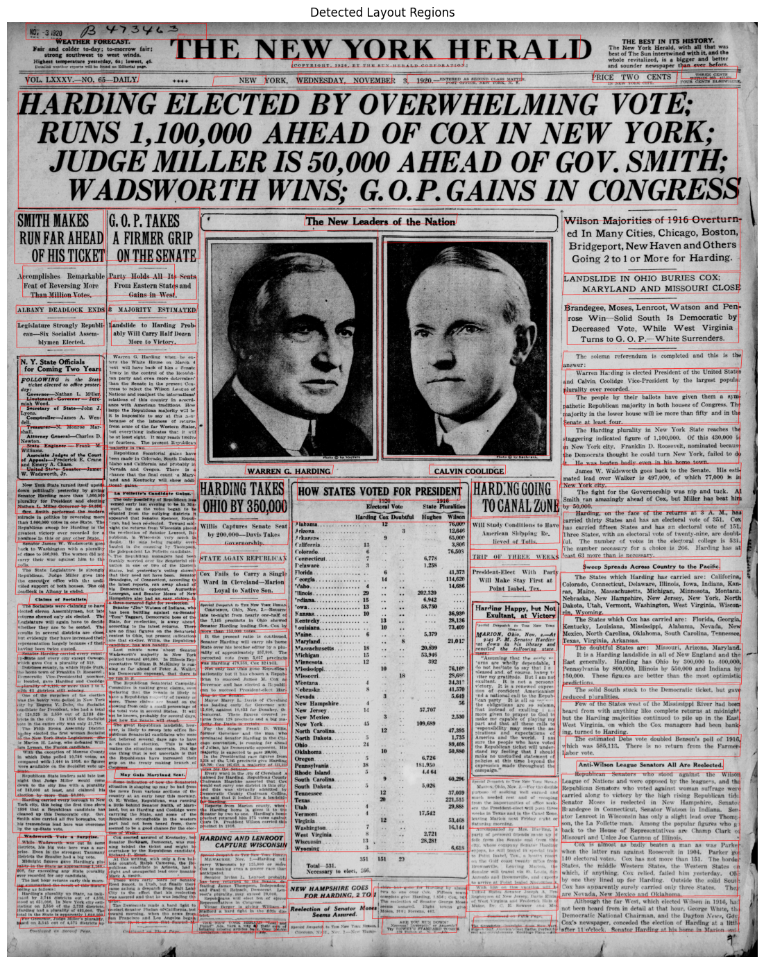
The algorithm has successfully ran and we can see red boxes around all of the major text sections, images and titles including tiny subheadings. This is an excellent tool and gives even more context to OCR.
OCR output often contains errors and requires cleaning. Post-processing can include:
Tokenization is the process of breaking down the raw text output generated from a scanned image or document into smaller, distinct, and manageable units called tokens. This simplifies data analysis, and Natural Language Processing (NLP) tasks.
We will use our simple newspaper column example from earlier. We have the sample text and we will first turn it into smaller tokens, and then stem and lemmatize the tokens. Here we use NLTK’s word_tokenize() which splits text into individual words and punctuation marks. This is different from the subword tokenization used by LLMs (like BPE), which breaks words into smaller pieces. For our purposes, word-level tokens are what we need for counting, stemming, and lemmatization.
sample_text = """
Twenty-Fifth Infantry Wins Athletic Honors

Champions of Six Regiments Compete in Exciting Finals of Tournament in Honolulu.

THE COLORED REGIMENT WINS.

Scores Nearly Half of All the Points Made by Combined Competitors Two Omaha Boys in Contest.
"""

tokens = word_tokenize(sample_text)
sentences = sent_tokenize(sample_text)

print("Tokenization Results:")
print(f"  Words: {len(tokens)}")
print(f"  Sentences: {len(sentences)}")
print(f"\nFirst 20 tokens: {tokens[:20]}")
Tokenization Results:
Words: 40
Sentences: 3
First 20 tokens: ['Twenty-Fifth', 'Infantry', 'Wins', 'Athletic', 'Honors', 'Champions', 'of', 'Six', 'Regiments', 'Compete', 'in', 'Exciting', 'Finals', 'of', 'Tournament', 'in', 'Honolulu', '.', 'THE', 'COLORED']The tokens here are just words as we are giving the raw correct text to the function, there is no OCR required, if it was complex OCR like with the handwritten letter the tokens that the model uses might be a little different from words.
Next we will run stemming and lemmatization on our tokens. “Stemming and lemmatization are text preprocessing techniques that reduce the inflected forms of words across a text data set to one common root word or dictionary form, also known as a “lemma” in computational linguistics.””
stemmer = PorterStemmer()
lemmatizer = WordNetLemmatizer()

test_words = ['running', 'competed', 'competitors', 'athletics', 'winning']

print("\nStemming vs Lemmatization:")
for word in test_words:
    stem = stemmer.stem(word)
    lemma = lemmatizer.lemmatize(word)
    print(f"  {word:15} -> Stem: {stem:12} | Lemma: {lemma}")
Stemming vs Lemmatization:
  running         -> Stem: run          | Lemma: running
  competed        -> Stem: compet       | Lemma: competed
  competitors     -> Stem: competitor   | Lemma: competitor
  athletics       -> Stem: athlet       | Lemma: athletics
  winning         -> Stem: win          | Lemma: winning
Stemming can be very useful for text analysis as all conjugations and versions of similar words are reduced to the root stem. It is vital for many Natural Language Processing techniques.
Converting OCR output to structured formats enables downstream analysis:
We make a function to save the .json output of our OCR.
#Create a structured JSON output from OCR results.
def create_structured_output(text, ocr_data_df, source_file, ocr_engine="easyocr"):
words = word_tokenize(text)
sentences = sent_tokenize(text)
output = {
"metadata": {
"source_file": source_file,
"ocr_engine": ocr_engine,
"total_characters": len(text),
"total_words": len(words),
"total_sentences": len(sentences),
"average_confidence": float(ocr_data_df['conf'].mean()) if 'conf' in ocr_data_df else None
},
"text": text.strip(),
"sentences": sentences,
"word_count_by_confidence": {
"high (90-100)": len(ocr_data_df[ocr_data_df['conf'] >= 90]),
"medium (70-89)": len(ocr_data_df[(ocr_data_df['conf'] >= 70) & (ocr_data_df['conf'] < 90)]),
"low (< 70)": len(ocr_data_df[ocr_data_df['conf'] < 70])
}
}
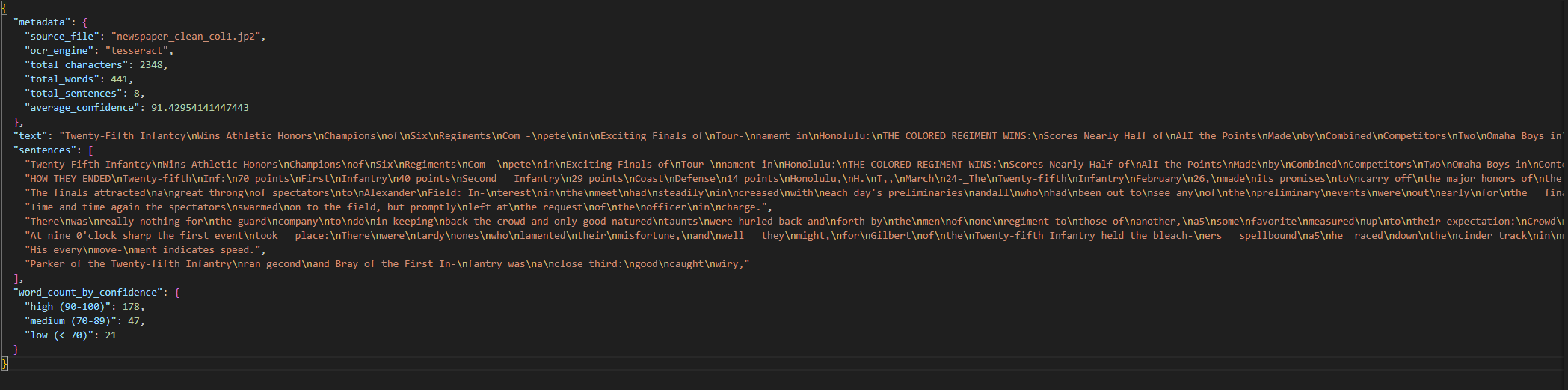
return outputThis will be for our simple newspaper column example:
structured = create_structured_output(extracted_text, ocr_df, "newspaper_clean_col1.jp2")

with open('output/document.json', 'w') as f:
    json.dump(structured, f, indent=2)

print("Structured Output:")
print(json.dumps(structured['metadata'], indent=2))
print(f"\nWord count by confidence: {structured['word_count_by_confidence']}")
print(f"\nSaved to: output/document.json")
Structured Output:
{
"source_file": "newspaper_clean_col1.jp2",
"ocr_engine": "easyocr",
"total_characters": 2348,
"total_words": 441,
"total_sentences": 8,
"average_confidence": 91.42954141447443
}
Word count by confidence: {'high (90-100)': 178, 'medium (70-89)': 47, 'low (< 70)': 21}
Saved to: output/document.jsonA .json is less human-readable than a .txt, but it is excellent for machine processing and programming tasks. Here what our .json looks like:
.json files are great tools for Natural Language Processing (NLP) techniques examples of which are:
For hands-on examples of several of these techniques, see the prAxIs Text Embeddings Workshop module.
For high-value documents, Large Language Models can correct OCR errors using contextual understanding that rule-based methods lack.
The cell below requires an ANTHROPIC_API_KEY environment variable set in your shell before launching the notebook. It calls Claude Haiku 4.5 and costs roughly $0.001 per run on a page of text. The code is commented out by default to avoid accidental API charges.
# LLM-based OCR correction with Claude Haiku 4.5
# Requires: ANTHROPIC_API_KEY env var.
#
# import anthropic
#
# client = anthropic.Anthropic()          # reads ANTHROPIC_API_KEY from env
#
# correction_prompt = (
#     "The following text was extracted from a historical newspaper using OCR. "
#     "Please correct any obvious OCR errors while preserving the original meaning "
#     "and historical language. Do not modernize spelling or grammar.\n\n"
#     "OCR TEXT:\n"
#     f"{extracted_text}\n\n"
#     "CORRECTED TEXT:"
# )
#
# message = client.messages.create(
#     model="claude-haiku-4-5",
#     max_tokens=2048,
#     messages=[{"role": "user", "content": correction_prompt}],
# )
#
# corrected_text = message.content[0].text
#
# # ── Display results ──────────────────────────────────────────────────
# print("=== Corrected Text ===\n")
# print(corrected_text)
#
# # ── Before / after snippet comparison ────────────────────────────────
# snippet_len = 500
# print("\n\n=== Before / After Comparison (first 500 chars) ===")
# print(f"\nBEFORE (raw OCR):\n{extracted_text[:snippet_len]}")
# print(f"\nAFTER  (LLM corrected):\n{corrected_text[:snippet_len]}")
Here is the output from running the cell above on our EasyOCR newspaper extraction (first 5 sentences shown):
=== Corrected Text ===

Twenty-Fifth Infantry Wins Athletic Honors

Champions of Six Regiments Compete in Exciting Finals of Tournament in Honolulu.

THE COLORED REGIMENT WINS.

Scores Nearly Half of All the Points Made by Combined Competitors Two Omaha Boys in Contest.

HOW THEY ENDED
Twenty-fifth Inf. ..................... 70 points
First Infantry ........................ 40 points
Second Infantry ....................... 29 points
Coast Defense ......................... 14 points

Honolulu, H. T., March 24—The Twenty-fifth Infantry February 26, made good its
promises to carry off the major honors of the big military athletic meet, finishing
in the finals against three other regiments with seventy points to its credit out
of a total of one hundred and fifty-four.
The LLM corrected several common OCR errors: Infantcy → Infantry, AlI → All, T,, → T.,, 24-_The → 24—The, and rejoined hyphenated line breaks (Com-pete → Compete, Tour-nament → Tournament). It also replaced colons with periods where appropriate and reconstructed the tabular score layout.
LLM corrections can catch errors that rule-based methods miss, though they carry a small risk of hallucinating plausible text that was not in the original document.
Evaluating OCR accuracy requires comparing extracted text against a known “ground truth.” We use two standard metrics:
We first load our correct .txt version of the newspaper column.
with open("data/simple/ground_truth_clean.txt", "r") as f:
    ground_truth = f.read()

print("Ground Truth (first 500 characters):")
print(ground_truth[:500])
Ground Truth (first 500 characters):
Twenty-Fifth Infantry Wins Athletic Honors
Champions of Six Regiments Compete in Exciting Finals of Tournament in Honolulu.
THE COLORED REGIMENT WINS.
Scores Nearly Half of All the Points Made by Combined Competitors Two Omaha Boys in Contest.
HOW THEY ENDED
Twenty-fifth Inf. .....................70 points
First Infantry..........................40 points
Second Infantry ......................29 points
Coast Defense .........................14 points
Honolulu, H. T., March 24—The Twenty-fAnd then we compare it with our EasyOCR output to see how the model performed.
gt_normalized = ground_truth.lower().strip()
ocr_normalized = extracted_text.lower().strip()

word_error_rate = wer(gt_normalized, ocr_normalized)
char_error_rate = cer(gt_normalized, ocr_normalized)

print("OCR Evaluation Metrics:")
print(f"\nWord Error Rate (WER):      {word_error_rate:.2%}")
print(f"Character Error Rate (CER): {char_error_rate:.2%}")
print(f"\nWord Accuracy:      {1 - word_error_rate:.2%}")
print(f"Character Accuracy: {1 - char_error_rate:.2%}")
OCR Evaluation Metrics:
Word Error Rate (WER): 80.51%
Character Error Rate (CER): 17.34%
Word Accuracy: 19.49%
Character Accuracy: 82.66%Interpreting Error Rates:
We can see that there are lots of errors from the EasyOCR output with only ~20% of words being correct and ~17% of characters being incorrect. Much of this error comes from how WER and CER are computed — differences in reading order, line breaks, and whitespace between the OCR output and ground truth all count as errors, even when the characters themselves were read correctly. This is why confidence was 91.4% but word accuracy is much lower.
We can use confidence scores to automatically flag words that likely need manual review. We set a threshold (in this case 70%), and we flag all other. These could also be fed into a LLM for editing.
low_conf_threshold = 70
low_conf_words = ocr_df[ocr_df['conf'] < low_conf_threshold][['text', 'conf']]

print(f"Words with confidence below {low_conf_threshold}%:")
print(f"  Total flagged: {len(low_conf_words)} out of {len(ocr_df)} ({len(low_conf_words)/len(ocr_df):.1%})")

if len(low_conf_words) > 0:
    print("\n  Sample low-confidence words:")
    display(low_conf_words.head(20))
Words with confidence below 70%:
Total flagged: 21 out of 246 (8.5%)
Sample low-confidence words:| text | conf | |
|---|---|---|
| 0 | Twenty-Fifth Infantcy | 62.461939 |
| 14 | Scores Nearly Half of | 68.373654 |
| 15 | AlI the Points | 53.332837 |
| 30 | Second Infantry | 64.370979 |
| 36 | H. | 22.868835 |
| 37 | T,, | 65.192774 |
| 39 | 24-_The | 21.203665 |
| 60 | its credit | 61.451588 |
| 82 | equal | 52.342412 |
| 87 | world. | 58.739307 |
| 99 | had | 57.016563 |
| 138 | charge. | 59.880112 |
| 157 | another, | 63.084649 |
| 158 | a5 | 38.334483 |
| 164 | their expectation: | 48.727530 |
| 169 | took place: | 48.095689 |
| 184 | the | 53.323942 |
| 186 | ers spellbound | 65.892382 |
| 187 | a5 | 67.793630 |
| 188 | he raced | 56.961843 |
We have a list of our worst text regions. With many of them being incorrect or just partial segments.
In this cell we will clear the demo images and cache for notebook performace.
# cleanup demo images from Parts 1-3 and clear Jupyter output cache
del img, img_with_boxes, surya_img, surya_result, surya_results
del letter_pages, letter_img, surya_hw_img, surya_hw_result, surya_hw_results
del easyocr_hw_results
del ubc_img, ubc_gray, ubc_binary, ubc_enhanced
del menu_img, menu_gray
del noisy_img, noisy_gray, otsu_binary
del noisy_notext, noisy_notext_gray, denoised_notext
del noisy_text, noisy_text_gray, denoised_text
del skewed_img, deskewed
del multicolumn_img, multicolumn_pil
get_ipython().history_manager.output_hist.clear()
gc.collect()
if torch.cuda.is_available():
torch.cuda.empty_cache()Parts 1–3 used curated, relatively clean sample images. Real archival documents are messier: faded ink, unusual fonts, handwritten annotations, and centuries of wear. We have seen different OCR models along with many techniques, in this section we put it all together into a full OCR workflow which we run on two different historical documents spanning different eras and formats.
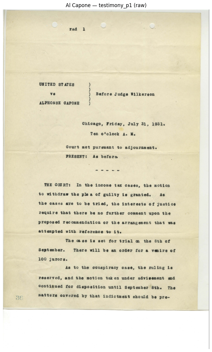
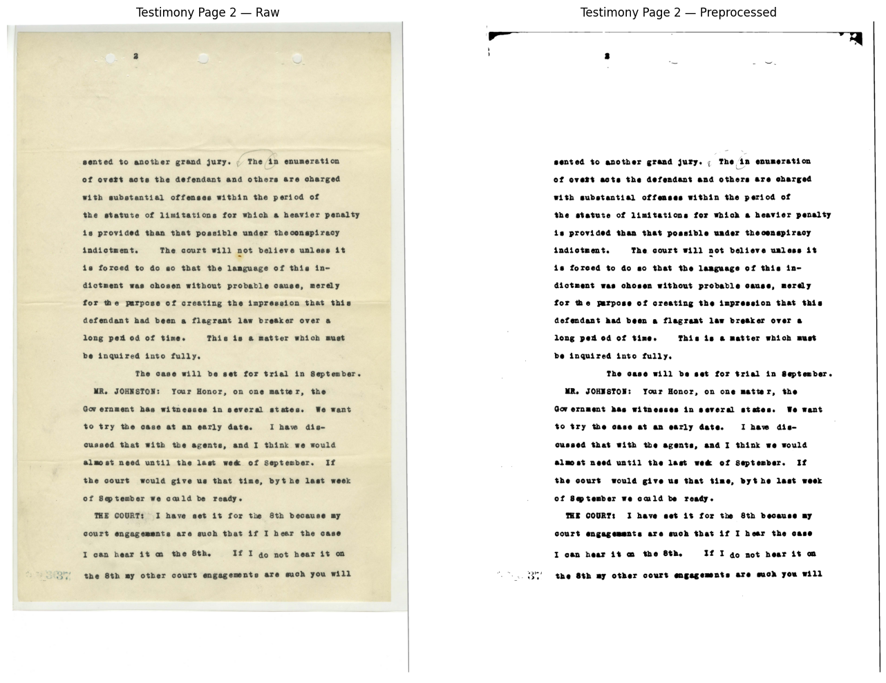
Our first real-world documents come from the Al Capone tax evasion case (1931). Legal documents of this era were typically typewritten, which should be favorable for OCR; but the scan quality and age of the documents introduce challenges. We have two items from this collection: the verdict (a GIF scan) and the first two pages of witness testimony (a PDF).
alcapone_verdict_raw = load_image("data/alcapone/alcapone_verdict.gif")

testimony_pages = convert_from_path(
    "data/alcapone/alcapone_testimony.pdf",
    dpi=300,
    first_page=1,
    last_page=2,
)
alcapone_testimony_p1_raw = np.array(testimony_pages[0])
alcapone_testimony_p2_raw = np.array(testimony_pages[1])

alcapone_documents = {
    "verdict": alcapone_verdict_raw,
    "testimony_p1": alcapone_testimony_p1_raw,
    "testimony_p2": alcapone_testimony_p2_raw,
}

for label, img in alcapone_documents.items():
    display_image(img, title=f"Al Capone — {label} (raw)", figsize=(10, 12))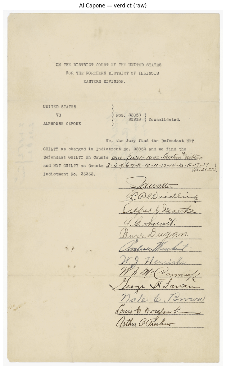
We can see that most of the text is written on a typewriter, and we have testimonial signatures on the first page.
Before running OCR we chain the same techniques introduced in Part 3 into a single pipeline function. The ordering matters: we convert to grayscale first (required by all subsequent steps), deskew to correct any rotation, denoise to remove speckle, apply CLAHE to boost local contrast, and finally binarize with Otsu’s method to produce a clean black-and-white image.
# our pre-processing pipeline (reuses a single array to save memory)
def preprocess_for_ocr(image):
    img = cv2.cvtColor(image, cv2.COLOR_RGB2GRAY)
    img, angle = deskew(img)
    img = cv2.fastNlMeansDenoising(img, h=10)
    clahe = cv2.createCLAHE(clipLimit=2.0, tileGridSize=(8, 8))
    img = clahe.apply(img)
    _, img = cv2.threshold(img, 0, 255, cv2.THRESH_BINARY + cv2.THRESH_OTSU)
return img, anglealcapone_preprocessed = {}
for label, img in alcapone_documents.items():
processed, angle = preprocess_for_ocr(img)
alcapone_preprocessed[label] = processed
print(f"{label}: detected skew angle = {angle:.2f}°")
display_images_side_by_side(
alcapone_documents["verdict"], alcapone_preprocessed["verdict"],
"Verdict — Raw", "Verdict — Preprocessed", figsize=(14, 10))
display_images_side_by_side(
alcapone_documents["testimony_p1"], alcapone_preprocessed["testimony_p1"],
"Testimony Page 1 — Raw", "Testimony Page 1 — Preprocessed", figsize=(14, 10))
display_images_side_by_side(
alcapone_documents["testimony_p2"], alcapone_preprocessed["testimony_p2"],
"Testimony Page 2 — Raw", "Testimony Page 2 — Preprocessed", figsize=(14, 10))verdict: detected skew angle = 0.00°
testimony_p1: detected skew angle = 0.00°
testimony_p2: detected skew angle = 0.00°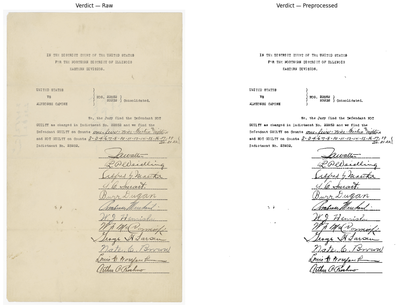
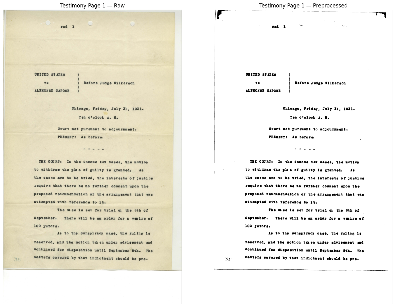
The output is much clearer with minimal noise and just black text on a white background. This will vastly improve OCR quality.
Before running OCR, we use Surya’s LayoutPredictor (Section 3.2) to identify document regions (Text, Table, SectionHeader, etc). Rather than feeding the entire page to the OCR engine and hoping it avoids non-text areas, we extract only the text-bearing regions and process them in reading order. This produces cleaner results because the recognizer never sees figures, decorations, or blank margins. For large batches this will also reduce computation time.
TEXT_LABELS = {"Text", "SectionHeader", "Title", "Caption", "Table",
               "ListItem", "Footnote", "PageHeader", "PageFooter"}

foundation_predictor = FoundationPredictor(checkpoint=settings.LAYOUT_MODEL_CHECKPOINT)
layout_predictor = LayoutPredictor(foundation_predictor)

alcapone_layouts = {}

for label, processed_img in alcapone_preprocessed.items():
    pil_img = Image.fromarray(cv2.cvtColor(processed_img, cv2.COLOR_GRAY2RGB))
    layout_results = layout_predictor([pil_img])
    layout = layout_results[0]
    alcapone_layouts[label] = layout

    print(f"{label}: {len(layout.bboxes)} regions detected")
    for box in layout.bboxes:
        marker = "*" if box.label in TEXT_LABELS else " "
        print(f"  {marker} [{box.label}] position {box.position}, confidence {box.confidence:.2%}")

    annotated = copy.deepcopy(pil_img)
    draw = ImageDraw.Draw(annotated)
    for box in layout.bboxes:
        poly = [(int(p[0]), int(p[1])) for p in box.polygon]
        color = "green" if box.label in TEXT_LABELS else "red"
        draw.line(poly + [poly[0]], fill=color, width=4)
        draw.text((poly[0][0], poly[0][1] - 14), f"{box.label} ({box.position})", fill=color)

    display_image(np.array(annotated), title=f"{label} — Layout Regions (green = OCR, red = skip)", figsize=(10, 12))
    print()

del layout_predictor, foundation_predictor
gc.collect()
if torch.cuda.is_available():
    torch.cuda.empty_cache()
Recognizing Layout: 0%| | 0/1 [00:00<?, ?it/s]Recognizing Layout: 100%|██████████| 1/1 [00:10<00:00, 10.97s/it]Recognizing Layout: 100%|██████████| 1/1 [00:10<00:00, 10.98s/it]verdict: 4 regions detected
* [SectionHeader] position 0, confidence 88.45%
[Form] position 1, confidence 67.06%
* [Text] position 2, confidence 69.19%
* [Text] position 3, confidence 79.06%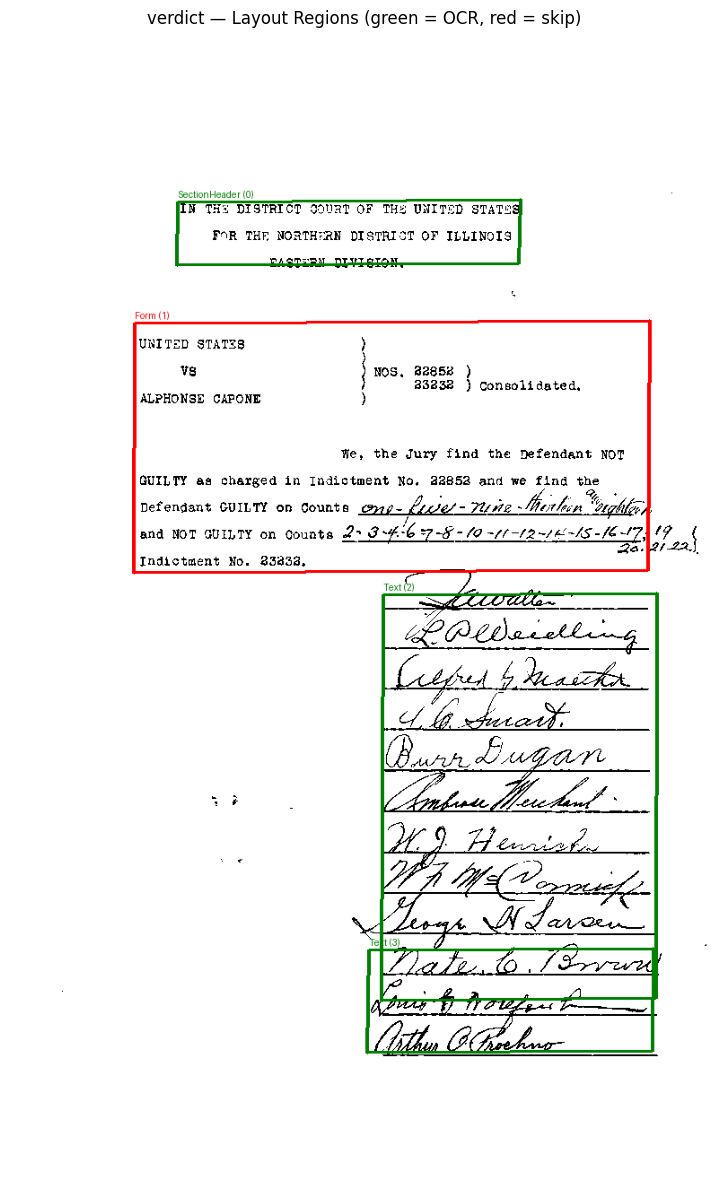
Recognizing Layout: 0%| | 0/1 [00:00<?, ?it/s]Recognizing Layout: 100%|██████████| 1/1 [00:11<00:00, 11.92s/it]Recognizing Layout: 100%|██████████| 1/1 [00:11<00:00, 11.94s/it]testimony_p1: 11 regions detected
* [PageHeader] position 0, confidence 92.59%
* [Text] position 1, confidence 96.97%
* [Text] position 2, confidence 99.97%
* [Text] position 3, confidence 99.95%
* [Text] position 4, confidence 99.89%
* [Text] position 5, confidence 99.96%
* [Text] position 6, confidence 99.99%
* [Text] position 7, confidence 99.96%
* [Text] position 8, confidence 99.99%
* [Text] position 9, confidence 99.95%
* [PageFooter] position 10, confidence 68.48%
Recognizing Layout: 0%| | 0/1 [00:00<?, ?it/s]Recognizing Layout: 100%|██████████| 1/1 [00:11<00:00, 11.58s/it]Recognizing Layout: 100%|██████████| 1/1 [00:11<00:00, 11.58s/it]testimony_p2: 3 regions detected
* [Text] position 0, confidence 97.47%
* [Text] position 1, confidence 99.98%
* [Text] position 2, confidence 99.95%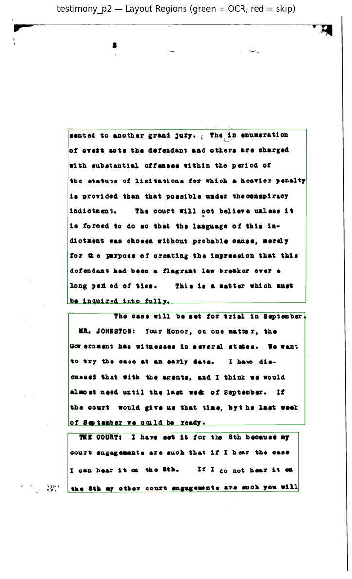
We can see green and red boxes around regions of interest in our documents. This improves our OCR quality by giving the OCR model information on what to expect in each section (text, section header, Table, Footnote), and how to interpret and analyze this text.
Now we run Surya’s recognition on only the text-bearing regions identified above, in reading order. For each region we crop the preprocessed image using the layout bounding box, run OCR on that crop, and collect the results. This avoids feeding blank margins, decorative elements, or non-text areas to the model.
foundation_predictor = FoundationPredictor()
rec_predictor = RecognitionPredictor(foundation_predictor)
det_predictor = DetectionPredictor()

alcapone_ocr_results = {}

for label, processed_img in alcapone_preprocessed.items():
    layout = alcapone_layouts[label]
    text_boxes = sorted(
        [b for b in layout.bboxes if b.label in TEXT_LABELS],
        key=lambda b: b.position,
    )

    all_texts = []
    all_scores = []
    h, w = processed_img.shape[:2]

    for box in text_boxes:
        xs = [p[0] for p in box.polygon]
        ys = [p[1] for p in box.polygon]
        x1 = max(0, int(min(xs)))
        y1 = max(0, int(min(ys)))
        x2 = min(w, int(max(xs)))
        y2 = min(h, int(max(ys)))

        crop = processed_img[y1:y2, x1:x2]
        if crop.size == 0:
            continue

        pil_crop = Image.fromarray(cv2.cvtColor(crop, cv2.COLOR_GRAY2RGB))
        results = rec_predictor([pil_crop], det_predictor=det_predictor)
        result = results[0]

        all_texts.extend([line.text for line in result.text_lines])
        all_scores.extend([line.confidence for line in result.text_lines])

    full_text = " ".join(all_texts)

    alcapone_ocr_results[label] = {
        "texts": all_texts,
        "scores": all_scores,
        "full_text": full_text,
    }

    print(f"{label}:")
    print(f"  Text regions used: {len(text_boxes)} of {len(layout.bboxes)}")
    print(f"  Lines detected   : {len(all_texts)}")
    print(f"  Avg confidence   : {np.mean(all_scores):.2%}" if all_scores else "  Avg confidence   : N/A")
    print(f"  Text preview     : {full_text[:300]}...\n")

del rec_predictor, det_predictor, foundation_predictor
gc.collect()
if torch.cuda.is_available():
    torch.cuda.empty_cache()
Detecting bboxes: 0%| | 0/1 [00:00<?, ?it/s]Detecting bboxes: 100%|██████████| 1/1 [00:02<00:00, 2.14s/it]Detecting bboxes: 100%|██████████| 1/1 [00:02<00:00, 2.14s/it]
Recognizing Text: 0%| | 0/3 [00:00<?, ?it/s]Recognizing Text: 33%|███▎ | 1/3 [00:03<00:07, 3.64s/it]Recognizing Text: 67%|██████▋ | 2/3 [00:05<00:02, 2.65s/it]Recognizing Text: 100%|██████████| 3/3 [00:06<00:00, 1.65s/it]Recognizing Text: 100%|██████████| 3/3 [00:06<00:00, 2.02s/it]
Detecting bboxes: 0%| | 0/1 [00:00<?, ?it/s]Detecting bboxes: 100%|██████████| 1/1 [00:01<00:00, 1.63s/it]Detecting bboxes: 100%|██████████| 1/1 [00:01<00:00, 1.63s/it]
Recognizing Text: 0%| | 0/11 [00:00<?, ?it/s]Recognizing Text: 9%|▉ | 1/11 [00:03<00:39, 3.95s/it]Recognizing Text: 18%|█▊ | 2/11 [00:04<00:18, 2.08s/it]Recognizing Text: 27%|██▋ | 3/11 [00:04<00:09, 1.19s/it]Recognizing Text: 64%|██████▎ | 7/11 [00:04<00:01, 2.83it/s]Recognizing Text: 82%|████████▏ | 9/11 [00:05<00:00, 3.60it/s]Recognizing Text: 100%|██████████| 11/11 [00:08<00:00, 1.25it/s]Recognizing Text: 100%|██████████| 11/11 [00:08<00:00, 1.22it/s]
Detecting bboxes: 0%| | 0/1 [00:00<?, ?it/s]Detecting bboxes: 100%|██████████| 1/1 [00:01<00:00, 1.88s/it]Detecting bboxes: 100%|██████████| 1/1 [00:01<00:00, 1.88s/it]
Recognizing Text: 0%| | 0/4 [00:00<?, ?it/s]Recognizing Text: 25%|██▌ | 1/4 [00:01<00:05, 1.95s/it]Recognizing Text: 50%|█████ | 2/4 [00:02<00:01, 1.03it/s]Recognizing Text: 75%|███████▌ | 3/4 [00:02<00:00, 1.27it/s]Recognizing Text: 100%|██████████| 4/4 [00:02<00:00, 1.38it/s]verdict:
Text regions used: 3 of 4
Lines detected : 18
Avg confidence : 80.02%
Text preview : IN THE DISTRICT COURT OF THE UNITED STATES FOR THE NORTHERN DISTRICT OF ILLINOIS PASTERN DIVISION _____ L'Oldeelling Sufrey & Martha 4. 6. Smart. (Burr Dugan Ambrou Mewhant. W.J. Henrich W/ Ma Vormely Leogs W. Larsen nate 6 Brown (a. ' & a. . . . . . . . . . . . . . . . . . nater 6.1 Inverse Louis ...
Detecting bboxes:   0%|          | 0/1 [00:00<?, ?it/s]Detecting bboxes: 100%|██████████| 1/1 [00:01<00:00,  1.48s/it]Detecting bboxes: 100%|██████████| 1/1 [00:01<00:00,  1.48s/it]
Recognizing Text:   0%|          | 0/2 [00:00<?, ?it/s]Recognizing Text:  50%|█████     | 1/2 [00:00<00:00,  1.94it/s]Recognizing Text: 100%|██████████| 2/2 [00:00<00:00,  3.87it/s]
Detecting bboxes:   0%|          | 0/1 [00:00<?, ?it/s]Detecting bboxes: 100%|██████████| 1/1 [00:01<00:00,  1.55s/it]Detecting bboxes: 100%|██████████| 1/1 [00:01<00:00,  1.55s/it]
Recognizing Text:   0%|          | 0/1 [00:00<?, ?it/s]Recognizing Text: 100%|██████████| 1/1 [00:01<00:00,  1.35s/it]Recognizing Text: 100%|██████████| 1/1 [00:01<00:00,  1.35s/it]
Detecting bboxes:   0%|          | 0/1 [00:00<?, ?it/s]Detecting bboxes: 100%|██████████| 1/1 [00:01<00:00,  1.42s/it]Detecting bboxes: 100%|██████████| 1/1 [00:01<00:00,  1.42s/it]
Recognizing Text:   0%|          | 0/1 [00:00<?, ?it/s]Recognizing Text: 100%|██████████| 1/1 [00:00<00:00,  3.00it/s]Recognizing Text: 100%|██████████| 1/1 [00:00<00:00,  3.00it/s]
Detecting bboxes:   0%|          | 0/1 [00:00<?, ?it/s]Detecting bboxes: 100%|██████████| 1/1 [00:01<00:00,  1.79s/it]Detecting bboxes: 100%|██████████| 1/1 [00:01<00:00,  1.79s/it]
Recognizing Text:   0%|          | 0/1 [00:00<?, ?it/s]Recognizing Text: 100%|██████████| 1/1 [00:02<00:00,  2.04s/it]Recognizing Text: 100%|██████████| 1/1 [00:02<00:00,  2.04s/it]
Detecting bboxes:   0%|          | 0/1 [00:00<?, ?it/s]Detecting bboxes: 100%|██████████| 1/1 [00:01<00:00,  1.57s/it]Detecting bboxes: 100%|██████████| 1/1 [00:01<00:00,  1.57s/it]
Recognizing Text:   0%|          | 0/1 [00:00<?, ?it/s]Recognizing Text: 100%|██████████| 1/1 [00:01<00:00,  1.96s/it]Recognizing Text: 100%|██████████| 1/1 [00:01<00:00,  1.96s/it]
Detecting bboxes:   0%|          | 0/1 [00:00<?, ?it/s]Detecting bboxes: 100%|██████████| 1/1 [00:01<00:00,  1.44s/it]Detecting bboxes: 100%|██████████| 1/1 [00:01<00:00,  1.44s/it]
Recognizing Text:   0%|          | 0/2 [00:00<?, ?it/s]Recognizing Text:  50%|█████     | 1/2 [00:02<00:02,  2.42s/it]Recognizing Text: 100%|██████████| 2/2 [00:03<00:00,  1.71s/it]Recognizing Text: 100%|██████████| 2/2 [00:03<00:00,  1.81s/it]
Detecting bboxes:   0%|          | 0/1 [00:00<?, ?it/s]Detecting bboxes: 100%|██████████| 1/1 [00:01<00:00,  1.45s/it]Detecting bboxes: 100%|██████████| 1/1 [00:01<00:00,  1.45s/it]
Recognizing Text:   0%|          | 0/1 [00:00<?, ?it/s]Recognizing Text: 100%|██████████| 1/1 [00:03<00:00,  3.02s/it]Recognizing Text: 100%|██████████| 1/1 [00:03<00:00,  3.02s/it]
Detecting bboxes:   0%|          | 0/1 [00:00<?, ?it/s]Detecting bboxes: 100%|██████████| 1/1 [00:01<00:00,  1.48s/it]Detecting bboxes: 100%|██████████| 1/1 [00:01<00:00,  1.48s/it]
Recognizing Text:   0%|          | 0/6 [00:00<?, ?it/s]Recognizing Text:  17%|█▋        | 1/6 [00:08<00:44,  8.90s/it]Recognizing Text:  33%|███▎      | 2/6 [00:10<00:18,  4.63s/it]Recognizing Text:  50%|█████     | 3/6 [00:10<00:07,  2.57s/it]Recognizing Text:  67%|██████▋   | 4/6 [00:11<00:03,  1.69s/it]Recognizing Text:  83%|████████▎ | 5/6 [00:11<00:01,  1.16s/it]Recognizing Text: 100%|██████████| 6/6 [00:11<00:00,  1.87s/it]
Detecting bboxes:   0%|          | 0/1 [00:00<?, ?it/s]Detecting bboxes: 100%|██████████| 1/1 [00:01<00:00,  1.45s/it]Detecting bboxes: 100%|██████████| 1/1 [00:01<00:00,  1.45s/it]
Recognizing Text:   0%|          | 0/3 [00:00<?, ?it/s]Recognizing Text:  33%|███▎      | 1/3 [00:02<00:05,  2.84s/it]Recognizing Text:  67%|██████▋   | 2/3 [00:05<00:02,  2.71s/it]Recognizing Text: 100%|██████████| 3/3 [00:06<00:00,  1.91s/it]Recognizing Text: 100%|██████████| 3/3 [00:06<00:00,  2.14s/it]
Detecting bboxes:   0%|          | 0/1 [00:00<?, ?it/s]Detecting bboxes: 100%|██████████| 1/1 [00:01<00:00,  1.45s/it]Detecting bboxes: 100%|██████████| 1/1 [00:01<00:00,  1.45s/it]
Recognizing Text:   0%|          | 0/4 [00:00<?, ?it/s]Recognizing Text:  25%|██▌       | 1/4 [00:07<00:23,  7.83s/it]Recognizing Text:  50%|█████     | 2/4 [00:08<00:07,  3.77s/it]Recognizing Text:  75%|███████▌  | 3/4 [00:08<00:02,  2.10s/it]Recognizing Text: 100%|██████████| 4/4 [00:08<00:00,  1.31s/it]Recognizing Text: 100%|██████████| 4/4 [00:08<00:00,  2.24s/it]
Detecting bboxes:   0%|          | 0/1 [00:00<?, ?it/s]Detecting bboxes: 100%|██████████| 1/1 [00:01<00:00,  1.39s/it]Detecting bboxes: 100%|██████████| 1/1 [00:01<00:00,  1.39s/it]
testimony_p1:
Text regions used: 11 of 11
Lines detected : 22
Avg confidence : 99.59%
Text preview : UNITED STATES Before Judge Wilkerson ALPHONSE CAPONE Chicago, Friday, July 31, 1931. Ten o'clock A. M. Court met pursuant to adjournment. THE COURT: In the income tax cases, the motion to withdraw the plea of guilty is granted. As the cases are to be tried, the interests of justice require that t...
Detecting bboxes:   0%|          | 0/1 [00:00<?, ?it/s]Detecting bboxes: 100%|██████████| 1/1 [00:01<00:00,  1.45s/it]Detecting bboxes: 100%|██████████| 1/1 [00:01<00:00,  1.45s/it]
Recognizing Text:   0%|          | 0/12 [00:00<?, ?it/s]Recognizing Text:   8%|▊         | 1/12 [00:12<02:20, 12.79s/it]Recognizing Text:  17%|█▋        | 2/12 [00:16<01:14,  7.42s/it]Recognizing Text:  25%|██▌       | 3/12 [00:16<00:37,  4.17s/it]Recognizing Text:  58%|█████▊    | 7/12 [00:17<00:06,  1.21s/it]Recognizing Text:  83%|████████▎ | 10/12 [00:17<00:01,  1.42it/s]Recognizing Text: 100%|██████████| 12/12 [00:17<00:00,  1.76it/s]Recognizing Text: 100%|██████████| 12/12 [00:17<00:00,  1.47s/it]
Detecting bboxes:   0%|          | 0/1 [00:00<?, ?it/s]Detecting bboxes: 100%|██████████| 1/1 [00:01<00:00,  1.49s/it]Detecting bboxes: 100%|██████████| 1/1 [00:01<00:00,  1.49s/it]
Recognizing Text:   0%|          | 0/8 [00:00<?, ?it/s]Recognizing Text:  12%|█▎        | 1/8 [00:09<01:06,  9.46s/it]Recognizing Text:  25%|██▌       | 2/8 [00:11<00:29,  4.86s/it]Recognizing Text:  50%|█████     | 4/8 [00:11<00:07,  1.85s/it]Recognizing Text:  62%|██████▎   | 5/8 [00:11<00:04,  1.40s/it]Recognizing Text:  75%|███████▌  | 6/8 [00:11<00:02,  1.01s/it]Recognizing Text:  88%|████████▊ | 7/8 [00:11<00:00,  1.36it/s]Recognizing Text: 100%|██████████| 8/8 [00:12<00:00,  1.69it/s]Recognizing Text: 100%|██████████| 8/8 [00:12<00:00,  1.51s/it]
Detecting bboxes:   0%|          | 0/1 [00:00<?, ?it/s]Detecting bboxes: 100%|██████████| 1/1 [00:01<00:00,  1.47s/it]Detecting bboxes: 100%|██████████| 1/1 [00:01<00:00,  1.47s/it]
Recognizing Text:   0%|          | 0/4 [00:00<?, ?it/s]Recognizing Text:  25%|██▌       | 1/4 [00:08<00:25,  8.59s/it]Recognizing Text:  50%|█████     | 2/4 [00:08<00:07,  3.60s/it]Recognizing Text:  75%|███████▌  | 3/4 [00:08<00:02,  2.05s/it]Recognizing Text: 100%|██████████| 4/4 [00:09<00:00,  1.32s/it]Recognizing Text: 100%|██████████| 4/4 [00:09<00:00,  2.28s/it]
testimony_p2:
Text regions used: 3 of 3
Lines detected : 24
Avg confidence : 99.15%
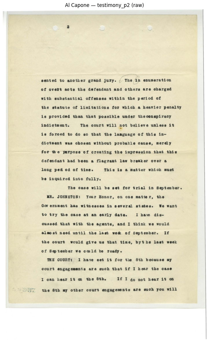
Text preview : sented to another grand jury. ( The in enumeration of overt acts the defendant and others are charged with substantial offenses within the period of the statute of limitations for which a heavier penalty is provided than that possible under the conspiracy indictment. The court will not believe unles...
We show the verdict (Page 1) and testimony page 2 (Page 3) here as representative examples; testimony page 1 is omitted for brevity but follows the same pattern.
Output Text Preview Page 1 (Verdict): “IN THE DISTRICT COURT OF THE UNITED STATES FOR THE NORTHERN DISTRICT OF ILLINOIS PASTERN DIVISION _____ L’Oldeelling Sufrey & Martha 4. 6. Smart. (Burr Dugan Ambrou Mewhant. W.J. Henrich W/ Ma Vormely Leogs W. Larsen nate 6 Brown”
Output Text Preview Page 3 (Testimony p2): “sented to another grand jury. ( The in enumeration of overt acts the defendant and others are charged with substantial offenses within the period of the statute of limitations for which a heavier penalty is provided than that possible under the conspiracy indictment.”
The model gives us a confidence value along with a preview of the text. The first page with the handwritten signatures has a much lower confidence than the rest of the document (we have seen previously how OCR struggles on handwritten text). The text preview also looks quite high quality. The third page specifically has a 99.09% confidence.
We divide every OCR line into three confidence tiers: high (>= 90%), medium (70–89%), and low (< 70%) - and flag the low-confidence lines for manual review. We could then send these low-confidence regions to an LLM for autocorrection.
summary_rows = []
for label, res in alcapone_ocr_results.items():
    scores = np.array(res["scores"])
    n = len(scores)
    high = int(np.sum(scores >= 0.90))
    medium = int(np.sum((scores >= 0.70) & (scores < 0.90)))
    low = int(np.sum(scores < 0.70))
    summary_rows.append({
        "Document": label,
        "Lines": n,
        "Avg Confidence": f"{np.mean(scores):.2%}" if n else "N/A",
        "High (>=90%)": f"{high} ({high/n:.0%})" if n else "0",
        "Medium (70-89%)": f"{medium} ({medium/n:.0%})" if n else "0",
        "Low (<70%)": f"{low} ({low/n:.0%})" if n else "0",
    })

summary_df = pd.DataFrame(summary_rows)
display(summary_df)

print("\n Low-confidence lines (< 70%) for manual review")
for label, res in alcapone_ocr_results.items():
    low_lines = [(t, s) for t, s in zip(res["texts"], res["scores"]) if s < 0.70]
    if low_lines:
        print(f"\n{label} ({len(low_lines)} lines):")
        for text, score in low_lines:
            print(f"  [{score:.2%}] {text}")
    else:
print(f"\n{label}: no low-confidence lines")| Document | Lines | Avg Confidence | High (>=90%) | Medium (70-89%) | Low (<70%) | |
|---|---|---|---|---|---|---|
| 0 | verdict | 18 | 80.02% | 7 (39%) | 6 (33%) | 5 (28%) |
| 1 | testimony_p1 | 22 | 99.59% | 22 (100%) | 0 (0%) | 0 (0%) |
| 2 | testimony_p2 | 24 | 99.15% | 23 (96%) | 1 (4%) | 0 (0%) |
 Low-confidence lines (< 70%) for manual review

verdict (5 lines):
  [39.98%] _____
  [53.30%] W/ Ma Vormely
  [63.75%] (a. ' & a. . . . . . . . . . . . . . . . . .
  [69.16%] nater 6.1
  [69.80%] Inverse

testimony_p1: no low-confidence lines

testimony_p2: no low-confidence lines
The handwritten signatures on the verdict are where we are having lower model performance.
Finally, we save each document’s OCR results in both JSON (machine-readable) and plain text formats. The create_surya_structured_output function mirrors the create_structured_output helper from Part 3, adapted for Surya’s line-level output with confidence scores.
def create_surya_structured_output(full_text, texts, scores, source_file):
    words = word_tokenize(full_text)
    sentences = sent_tokenize(full_text)
    scores_arr = np.array(scores)

    output = {
        "metadata": {
            "source_file": source_file,
            "ocr_engine": "surya",
            "total_lines": len(texts),
            "total_characters": len(full_text),
            "total_words": len(words),
            "total_sentences": len(sentences),
            "average_confidence": float(np.mean(scores_arr)) if len(scores_arr) else None,
        },
        "text": full_text.strip(),
        "sentences": sentences,
        "lines": [
            {"text": t, "confidence": float(s)} for t, s in zip(texts, scores)
        ],
        "confidence_distribution": {
            "high (>=90%)": int(np.sum(scores_arr >= 0.90)),
            "medium (70-89%)": int(np.sum((scores_arr >= 0.70) & (scores_arr < 0.90))),
            "low (<70%)": int(np.sum(scores_arr < 0.70)),
        },
    }
    return output

file_labels = {
    "verdict": "alcapone_verdict",
    "testimony_p1": "alcapone_testimony_p1",
    "testimony_p2": "alcapone_testimony_p2",
}

for label, res in alcapone_ocr_results.items():
    structured = create_surya_structured_output(
        res["full_text"], res["texts"], res["scores"],
        source_file=file_labels[label],
    )

    json_path = f"output/{file_labels[label]}.json"
    txt_path = f"output/{file_labels[label]}.txt"

    with open(json_path, "w", encoding="utf-8") as f:
        json.dump(structured, f, indent=2, ensure_ascii=False)

    with open(txt_path, "w", encoding="utf-8") as f:
        f.write(structured["text"])

    print(f"Saved: {json_path}  ({structured['metadata']['total_words']} words)")
    print(f"Saved: {txt_path}")
    print()
Saved: output/alcapone_verdict.json (77 words)
Saved: output/alcapone_verdict.txt
Saved: output/alcapone_testimony_p1.json (138 words)
Saved: output/alcapone_testimony_p1.txt
Saved: output/alcapone_testimony_p2.json (235 words)
Saved: output/alcapone_testimony_p2.txt
For the testimony pages we have a human transcription, which lets us compute the same WER and CER metrics introduced in section 3.4. This is the real test: confidence scores tell us what the model thinks, but error rates tell us what actually happened.
with open("data/alcapone/correct_text/correct_testimony.txt", "r") as f:
    testimony_ground_truth = f.read()

print("Ground truth (first 500 characters):")
print(testimony_ground_truth[:500])
Ground truth (first 500 characters):
UNITED STATES )
)
vs ) Before Judge Wilkerson
)
ALPHONSE CAPONE )
Chicago, Friday, July 31, 1931.
Ten o'clock A. M.
Court met pursuant to adjournment.
PRESENT: As before.
- - - - -
THE COURT: In the income tax cases, the motion
to withdraw the plea of guilty is granted. As
the cases are to be tried, the interestsWe can preview the ground truth testimony and then concatenate the OCR output from both testimony pages and compare against the full ground truth.
testimony_ocr_text = (
    alcapone_ocr_results["testimony_p1"]["full_text"]
    + " "
    + alcapone_ocr_results["testimony_p2"]["full_text"]
)

def normalize_for_comparison(text):
    text = text.lower().strip()
    text = re.sub(r'\s+', ' ', text)
    return text

gt_normalized = normalize_for_comparison(testimony_ground_truth)
ocr_normalized = normalize_for_comparison(testimony_ocr_text)

word_error_rate = wer(gt_normalized, ocr_normalized)
char_error_rate = cer(gt_normalized, ocr_normalized)

print("TESTIMONY OCR EVALUATION")
print(f"\nWord Error Rate (WER):      {word_error_rate:.2%}")
print(f"Word Accuracy:              {1 - word_error_rate:.2%}")
print(f"\nCharacter Error Rate (CER): {char_error_rate:.2%}")
print(f"Character Accuracy:         {1 - char_error_rate:.2%}")
TESTIMONY OCR EVALUATION
Word Error Rate (WER): 6.84%
Word Accuracy: 93.16%
Character Error Rate (CER): 2.84%
Character Accuracy: 97.16%The preprocessing into OCR into post-processing pipeline is now complete for the Al Capone documents. For the verdict we relied on confidence scores alone, but the testimony evaluation with ground truth gives us a concrete measure of how well the pipeline actually performed.
We can see that we have a low WER and CER. This is a good score, and could be improved further with post-processing techniques like LLM correction. This worked well for the typewritten case, but let’s try something even more ambitious.
# cleanup Al Capone data and clear Jupyter output cache
del alcapone_documents, alcapone_preprocessed, alcapone_layouts
del alcapone_ocr_results, testimony_ground_truth, testimony_ocr_text
get_ipython().history_manager.output_hist.clear()
gc.collect()
if torch.cuda.is_available():
torch.cuda.empty_cache()Our most challenging case: pages from medieval medical and astrological texts. Unlike the typewritten Al Capone documents, these are handwritten in medieval scripts with abbreviations, Latin text, and marginal annotations. We apply the same preprocessing, Surya OCR, confidence analysis, export pipeline used above. Here we do not have a ground truth and will have to rely on confidence scores and an eye test.
We will be using Cirogia vulgare. Ricettario. Antidotarium vulgare which was published between 1300 and 1350 in Latin and Medical/Astrological texts in English published between 1551 and 1553.
To be clear this is difficult for OCR and we are not expecting an excellent result using a relatively simple and non-computationally intensive model (Surya) that is not specifically trained for medieval text like this.
We load and display our documents:
medieval_chirurgia_raw = load_image("data/medieval_medical_manuscripts/cirogia_vulgare_1.jpg")
medieval_calendar_raw = load_image("data/medieval_medical_manuscripts/calendars_3.jpg")

medieval_documents = {
    "chirurgia_vulgare": medieval_chirurgia_raw,
    "calendar_3": medieval_calendar_raw,
}

for label, img in medieval_documents.items():
    display_image(img, title=f"Medieval — {label} (raw)", figsize=(10, 12))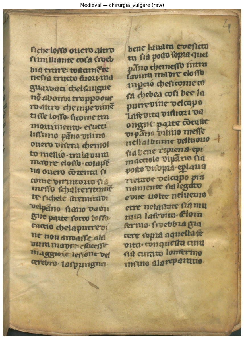
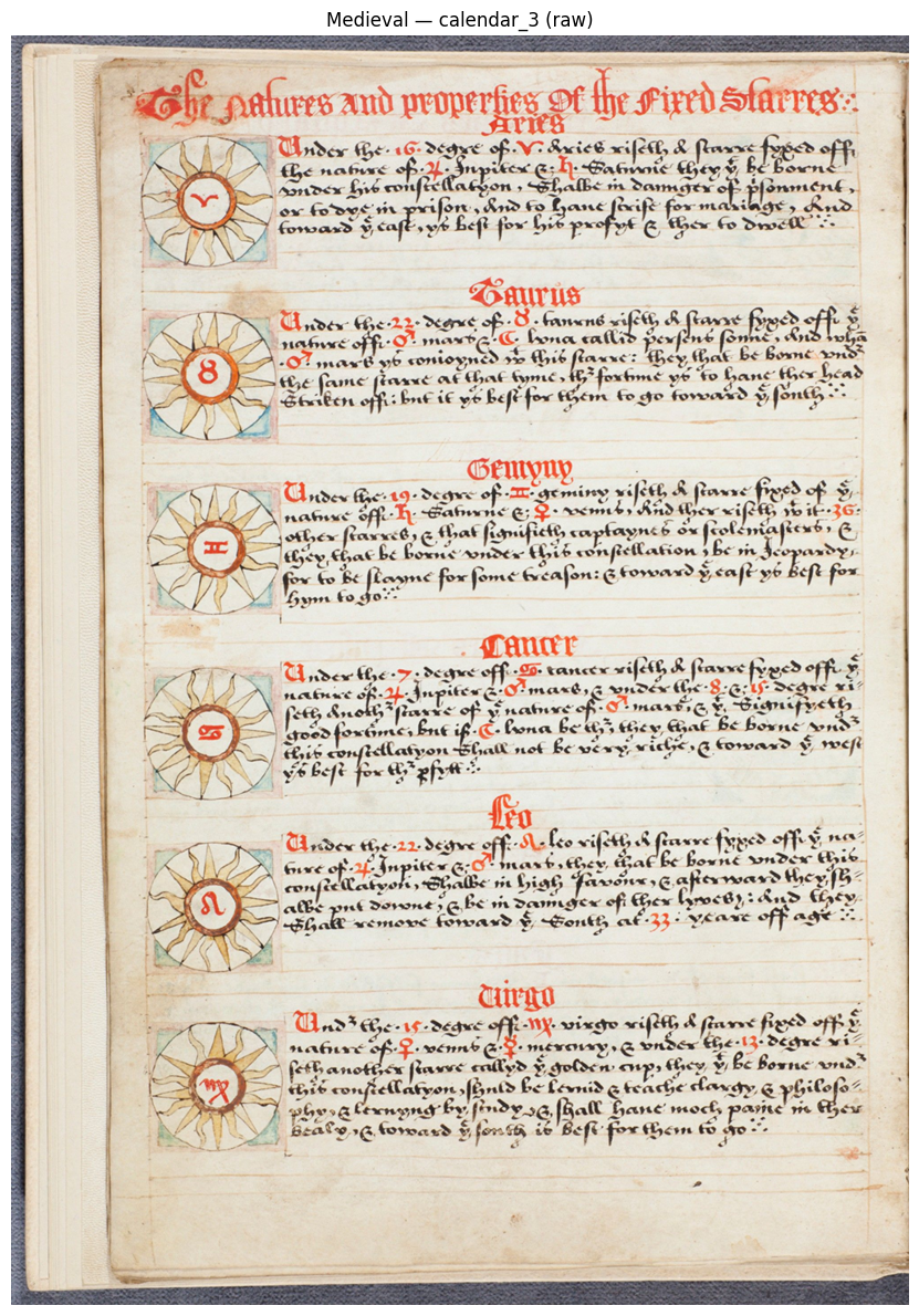
We reuse the preprocess_for_ocr pipeline defined in section 4.1. Medieval manuscripts may have significant skew from uneven binding and faded ink, so the deskew and CLAHE steps are especially important here.
medieval_preprocessed = {}
for label, img in medieval_documents.items():
    processed, angle = preprocess_for_ocr(img)
    medieval_preprocessed[label] = processed
    print(f"{label}: detected skew angle = {angle:.2f}°")

display_images_side_by_side(
    medieval_documents["chirurgia_vulgare"], medieval_preprocessed["chirurgia_vulgare"],
    "Chirurgia Vulgare — Raw", "Chirurgia Vulgare — Preprocessed", figsize=(14, 10)
)
display_images_side_by_side(
    medieval_documents["calendar_3"], medieval_preprocessed["calendar_3"],
    "Calendar 3 — Raw", "Calendar 3 — Preprocessed", figsize=(14, 10)
)
chirurgia_vulgare: detected skew angle = -1.00°
calendar_3: detected skew angle = -2.00°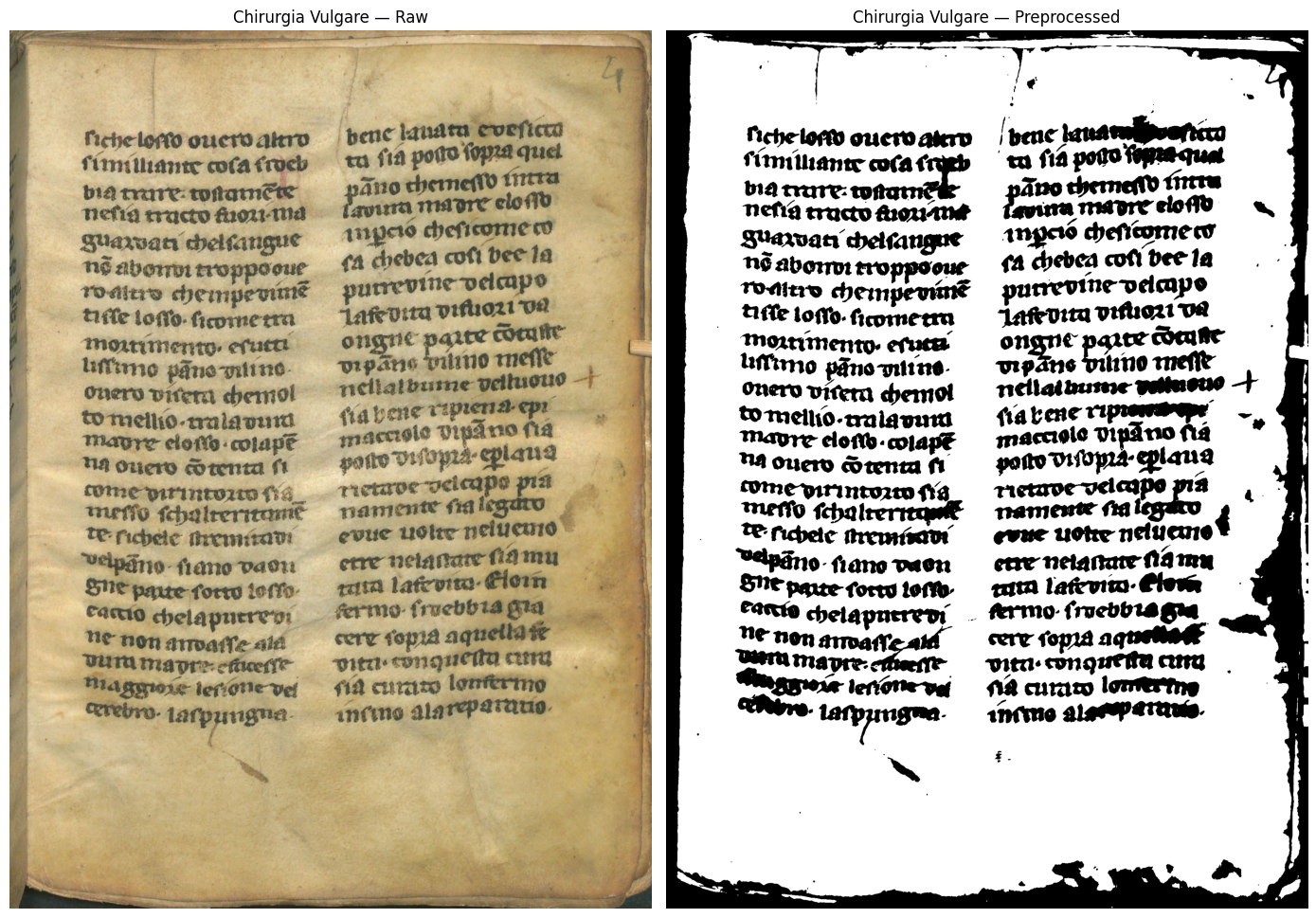
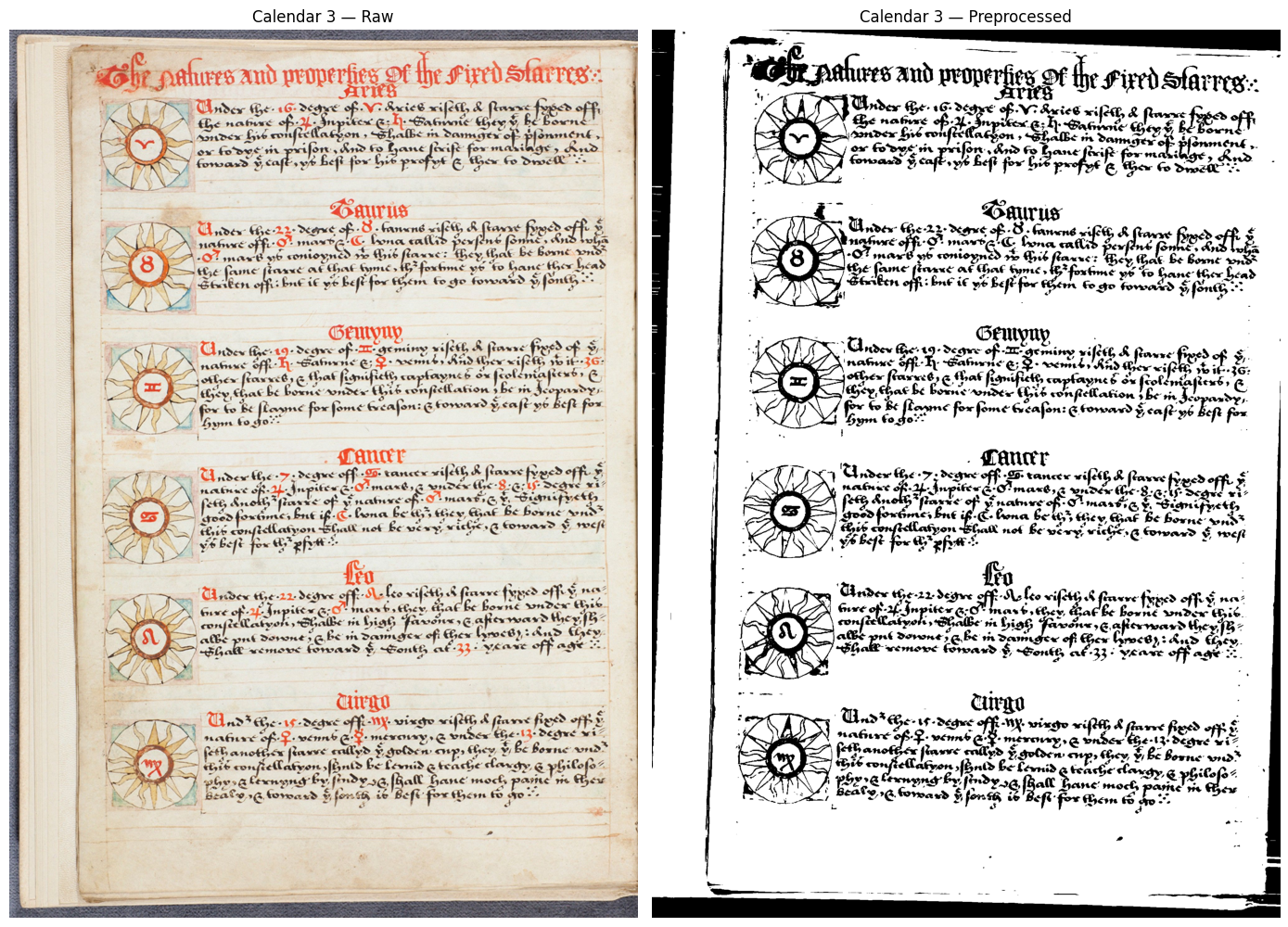
Once again the output is far clearer with minimal noise and black text on a pure white background.
Layout analysis on medieval manuscripts is especially valuable. These documents mix body text, marginal annotations, decorated initials, and tabular elements (the calendar page). By identifying regions first, we can feed only text-bearing areas to the OCR engine and skip illuminations and decorations that would produce garbage output.
foundation_predictor = FoundationPredictor(checkpoint=settings.LAYOUT_MODEL_CHECKPOINT)
layout_predictor = LayoutPredictor(foundation_predictor)

medieval_layouts = {}

for label, processed_img in medieval_preprocessed.items():
    pil_img = Image.fromarray(cv2.cvtColor(processed_img, cv2.COLOR_GRAY2RGB))
    layout_results = layout_predictor([pil_img])
    layout = layout_results[0]
    medieval_layouts[label] = layout

    print(f"--- {label}: {len(layout.bboxes)} regions detected ---")
    for box in layout.bboxes:
        marker = "*" if box.label in TEXT_LABELS else " "
        print(f"  {marker} [{box.label}] position {box.position}, confidence {box.confidence:.2%}")

    annotated = copy.deepcopy(pil_img)
    draw = ImageDraw.Draw(annotated)
    for box in layout.bboxes:
        poly = [(int(p[0]), int(p[1])) for p in box.polygon]
        color = "green" if box.label in TEXT_LABELS else "red"
        draw.line(poly + [poly[0]], fill=color, width=4)
        draw.text((poly[0][0], poly[0][1] - 14), f"{box.label} ({box.position})", fill=color)

    display_image(np.array(annotated), title=f"{label} — Layout Regions (green = OCR, red = skip)", figsize=(10, 12))
    print()

del layout_predictor, foundation_predictor
gc.collect()
if torch.cuda.is_available():
    torch.cuda.empty_cache()
Recognizing Layout: 0%| | 0/1 [00:00<?, ?it/s]Recognizing Layout: 100%|██████████| 1/1 [00:11<00:00, 11.77s/it]Recognizing Layout: 100%|██████████| 1/1 [00:11<00:00, 11.77s/it]--- chirurgia_vulgare: 2 regions detected ---
* [Text] position 0, confidence 99.73%
* [Text] position 1, confidence 99.62%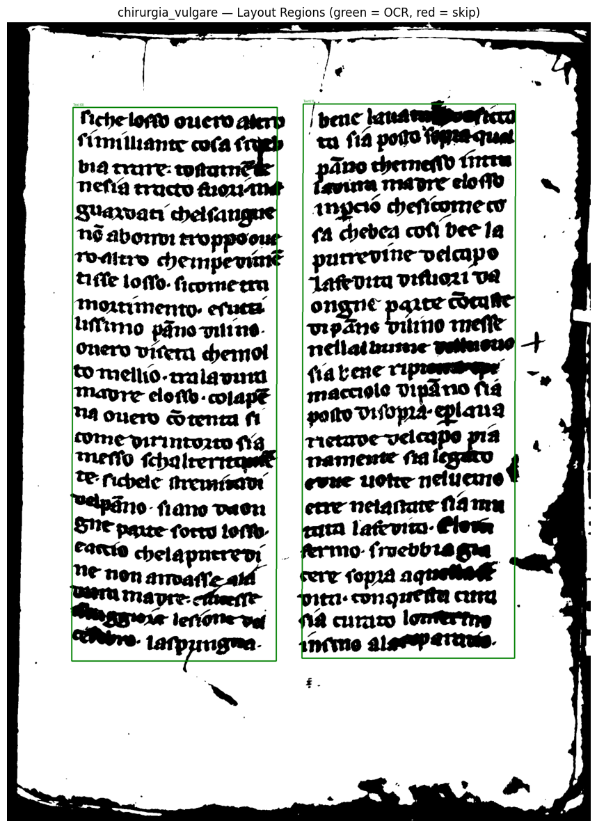
Recognizing Layout: 0%| | 0/1 [00:00<?, ?it/s]Recognizing Layout: 100%|██████████| 1/1 [00:12<00:00, 12.38s/it]Recognizing Layout: 100%|██████████| 1/1 [00:12<00:00, 12.38s/it]--- calendar_3: 13 regions detected ---
* [Text] position 0, confidence 53.27%
* [Text] position 1, confidence 54.22%
* [Text] position 2, confidence 98.65%
* [Text] position 3, confidence 55.33%
* [Text] position 4, confidence 97.67%
[Picture] position 5, confidence 57.38%
* [Text] position 6, confidence 98.95%
[Picture] position 7, confidence 81.46%
* [Text] position 8, confidence 99.75%
[Picture] position 9, confidence 89.71%
* [Text] position 10, confidence 99.89%
[Picture] position 11, confidence 84.52%
* [Text] position 12, confidence 99.37%
With our layout set we can run the proper OCR.
foundation_predictor = FoundationPredictor()
rec_predictor = RecognitionPredictor(foundation_predictor)
det_predictor = DetectionPredictor()

medieval_ocr_results = {}

for label, processed_img in medieval_preprocessed.items():
    layout = medieval_layouts[label]
    text_boxes = sorted(
        [b for b in layout.bboxes if b.label in TEXT_LABELS],
        key=lambda b: b.position,
    )

    all_texts = []
    all_scores = []
    h, w = processed_img.shape[:2]

    for box in text_boxes:
        xs = [p[0] for p in box.polygon]
        ys = [p[1] for p in box.polygon]
        x1 = max(0, int(min(xs)))
        y1 = max(0, int(min(ys)))
        x2 = min(w, int(max(xs)))
        y2 = min(h, int(max(ys)))

        crop = processed_img[y1:y2, x1:x2]
        if crop.size == 0:
            continue

        pil_crop = Image.fromarray(cv2.cvtColor(crop, cv2.COLOR_GRAY2RGB))
        results = rec_predictor([pil_crop], det_predictor=det_predictor)
        result = results[0]

        all_texts.extend([line.text for line in result.text_lines])
        all_scores.extend([line.confidence for line in result.text_lines])

    full_text = " ".join(all_texts)

    medieval_ocr_results[label] = {
        "texts": all_texts,
        "scores": all_scores,
        "full_text": full_text,
    }

    print(f"--- {label} ---")
    print(f"  Text regions used: {len(text_boxes)} of {len(layout.bboxes)}")
    print(f"  Lines detected   : {len(all_texts)}")
    print(f"  Avg confidence   : {np.mean(all_scores):.2%}" if all_scores else "  Avg confidence   : N/A")
    print(f"  Text preview     : {full_text[:300]}...\n")

del rec_predictor, det_predictor, foundation_predictor
gc.collect()
if torch.cuda.is_available():
    torch.cuda.empty_cache()
Detecting bboxes: 0%| | 0/1 [00:00<?, ?it/s]Detecting bboxes: 100%|██████████| 1/1 [00:04<00:00, 4.96s/it]Detecting bboxes: 100%|██████████| 1/1 [00:04<00:00, 4.96s/it]
Recognizing Text: 0%| | 0/22 [00:00<?, ?it/s]Recognizing Text: 5%|▍ | 1/22 [00:16<05:52, 16.80s/it]Recognizing Text: 23%|██▎ | 5/22 [00:17<00:43, 2.55s/it]Recognizing Text: 55%|█████▍ | 12/22 [00:17<00:08, 1.20it/s]Recognizing Text: 68%|██████▊ | 15/22 [00:17<00:04, 1.64it/s]Recognizing Text: 86%|████████▋ | 19/22 [00:17<00:01, 2.44it/s]Recognizing Text: 100%|██████████| 22/22 [00:17<00:00, 3.16it/s]Recognizing Text: 100%|██████████| 22/22 [00:17<00:00, 1.23it/s]
Detecting bboxes: 0%| | 0/1 [00:00<?, ?it/s]Detecting bboxes: 100%|██████████| 1/1 [00:02<00:00, 2.56s/it]Detecting bboxes: 100%|██████████| 1/1 [00:02<00:00, 2.56s/it]
Recognizing Text: 0%| | 0/22 [00:00<?, ?it/s]Recognizing Text: 5%|▍ | 1/22 [00:15<05:32, 15.85s/it]Recognizing Text: 9%|▉ | 2/22 [00:16<02:12, 6.65s/it]Recognizing Text: 18%|█▊ | 4/22 [00:16<00:45, 2.55s/it]Recognizing Text: 32%|███▏ | 7/22 [00:16<00:16, 1.13s/it]Recognizing Text: 64%|██████▎ | 14/22 [00:16<00:03, 2.44it/s]Recognizing Text: 82%|████████▏ | 18/22 [00:16<00:01, 3.51it/s]Recognizing Text: 91%|█████████ | 20/22 [00:17<00:00, 4.02it/s]Recognizing Text: 100%|██████████| 22/22 [00:19<00:00, 2.33it/s]Recognizing Text: 100%|██████████| 22/22 [00:19<00:00, 1.14it/s]--- chirurgia_vulgare ---
Text regions used: 2 of 2
Lines detected : 44
Avg confidence : 85.47%
Text preview : fichelosso ouesto aten similiance cola sinci bid trure whamest nesia tructo Avouani Suarvan chellangue no aborron troppooue roaltro chempevins tisse losso. sicometra mountmento, esuces listimo pāno vilins. onero vitera chemol to mellio-uniavum mattre elosso colape na ouero cotenta fi come dirintozeo...
Detecting bboxes:   0%|          | 0/1 [00:00<?, ?it/s]Detecting bboxes: 100%|██████████| 1/1 [00:01<00:00,  1.52s/it]Detecting bboxes: 100%|██████████| 1/1 [00:01<00:00,  1.52s/it]
Recognizing Text:   0%|          | 0/2 [00:00<?, ?it/s]Recognizing Text:  50%|█████     | 1/2 [00:10<00:10, 10.20s/it]Recognizing Text: 100%|██████████| 2/2 [00:15<00:00,  7.31s/it]Recognizing Text: 100%|██████████| 2/2 [00:15<00:00,  7.75s/it]
Detecting bboxes:   0%|          | 0/1 [00:00<?, ?it/s]Detecting bboxes: 100%|██████████| 1/1 [00:01<00:00,  1.47s/it]Detecting bboxes: 100%|██████████| 1/1 [00:01<00:00,  1.47s/it]
Recognizing Text:   0%|          | 0/2 [00:00<?, ?it/s]Recognizing Text:  50%|█████     | 1/2 [00:00<00:00,  1.56it/s]Recognizing Text: 100%|██████████| 2/2 [00:00<00:00,  3.12it/s]
Detecting bboxes:   0%|          | 0/1 [00:00<?, ?it/s]Detecting bboxes: 100%|██████████| 1/1 [00:01<00:00,  1.54s/it]Detecting bboxes: 100%|██████████| 1/1 [00:01<00:00,  1.54s/it]
Recognizing Text:   0%|          | 0/2 [00:00<?, ?it/s]Recognizing Text:  50%|█████     | 1/2 [00:14<00:14, 14.45s/it]Recognizing Text: 100%|██████████| 2/2 [00:19<00:00,  9.08s/it]Recognizing Text: 100%|██████████| 2/2 [00:19<00:00,  9.88s/it]
Detecting bboxes:   0%|          | 0/1 [00:00<?, ?it/s]Detecting bboxes: 100%|██████████| 1/1 [00:01<00:00,  1.40s/it]Detecting bboxes: 100%|██████████| 1/1 [00:01<00:00,  1.40s/it]
Recognizing Text:   0%|          | 0/2 [00:00<?, ?it/s]Recognizing Text:  50%|█████     | 1/2 [00:00<00:00,  1.54it/s]Recognizing Text: 100%|██████████| 2/2 [00:00<00:00,  2.69it/s]Recognizing Text: 100%|██████████| 2/2 [00:00<00:00,  2.42it/s]
Detecting bboxes:   0%|          | 0/1 [00:00<?, ?it/s]Detecting bboxes: 100%|██████████| 1/1 [00:01<00:00,  1.52s/it]Detecting bboxes: 100%|██████████| 1/1 [00:01<00:00,  1.52s/it]
Recognizing Text:   0%|          | 0/5 [00:00<?, ?it/s]Recognizing Text:  20%|██        | 1/5 [00:05<00:23,  5.98s/it]Recognizing Text:  40%|████      | 2/5 [00:11<00:17,  5.82s/it]Recognizing Text:  80%|████████  | 4/5 [00:12<00:02,  2.28s/it]Recognizing Text: 100%|██████████| 5/5 [00:18<00:00,  3.66s/it]Recognizing Text: 100%|██████████| 5/5 [00:18<00:00,  3.75s/it]
Detecting bboxes:   0%|          | 0/1 [00:00<?, ?it/s]Detecting bboxes: 100%|██████████| 1/1 [00:01<00:00,  1.53s/it]Detecting bboxes: 100%|██████████| 1/1 [00:01<00:00,  1.54s/it]
Recognizing Text:   0%|          | 0/3 [00:00<?, ?it/s]Recognizing Text:  33%|███▎      | 1/3 [00:06<00:12,  6.15s/it]Recognizing Text:  67%|██████▋   | 2/3 [00:12<00:06,  6.45s/it]Recognizing Text: 100%|██████████| 3/3 [00:29<00:00, 11.05s/it]Recognizing Text: 100%|██████████| 3/3 [00:29<00:00,  9.78s/it]
Detecting bboxes:   0%|          | 0/1 [00:00<?, ?it/s]Detecting bboxes: 100%|██████████| 1/1 [00:01<00:00,  1.58s/it]Detecting bboxes: 100%|██████████| 1/1 [00:01<00:00,  1.58s/it]
Recognizing Text:   0%|          | 0/6 [00:00<?, ?it/s]Recognizing Text:  17%|█▋        | 1/6 [00:06<00:32,  6.47s/it]Recognizing Text:  33%|███▎      | 2/6 [00:07<00:14,  3.52s/it]Recognizing Text:  50%|█████     | 3/6 [00:12<00:11,  3.92s/it]Recognizing Text:  67%|██████▋   | 4/6 [00:12<00:05,  2.51s/it]Recognizing Text:  83%|████████▎ | 5/6 [00:13<00:01,  1.78s/it]Recognizing Text: 100%|██████████| 6/6 [00:20<00:00,  3.63s/it]Recognizing Text: 100%|██████████| 6/6 [00:20<00:00,  3.40s/it]
Detecting bboxes:   0%|          | 0/1 [00:00<?, ?it/s]Detecting bboxes: 100%|██████████| 1/1 [00:01<00:00,  1.52s/it]Detecting bboxes: 100%|██████████| 1/1 [00:01<00:00,  1.52s/it]
Recognizing Text:   0%|          | 0/4 [00:00<?, ?it/s]Recognizing Text:  25%|██▌       | 1/4 [00:06<00:18,  6.11s/it]Recognizing Text:  50%|█████     | 2/4 [00:11<00:11,  5.80s/it]Recognizing Text:  75%|███████▌  | 3/4 [00:11<00:03,  3.20s/it]Recognizing Text: 100%|██████████| 4/4 [00:26<00:00,  7.60s/it]Recognizing Text: 100%|██████████| 4/4 [00:26<00:00,  6.54s/it]
Detecting bboxes:   0%|          | 0/1 [00:00<?, ?it/s]Detecting bboxes: 100%|██████████| 1/1 [00:01<00:00,  1.50s/it]Detecting bboxes: 100%|██████████| 1/1 [00:01<00:00,  1.50s/it]
Recognizing Text:   0%|          | 0/7 [00:00<?, ?it/s]Recognizing Text:  14%|█▍        | 1/7 [00:06<00:41,  6.97s/it]Recognizing Text:  29%|██▊       | 2/7 [00:12<00:30,  6.15s/it]Recognizing Text:  57%|█████▋    | 4/7 [00:13<00:07,  2.49s/it]Recognizing Text:  71%|███████▏  | 5/7 [00:13<00:03,  1.76s/it]Recognizing Text:  86%|████████▌ | 6/7 [00:13<00:01,  1.37s/it]Recognizing Text: 100%|██████████| 7/7 [00:13<00:00,  1.01it/s]Recognizing Text: 100%|██████████| 7/7 [00:13<00:00,  1.99s/it]
--- calendar_3 ---
Text regions used: 9 of 13
Lines detected : 33
Avg confidence : 71.58%
Text preview : The Pathures and properties Of the Fixed Starres. Ander the 16 degre of V. Snieb rifeth & forme topes offi<br>the nature of 4. Invites a hora constant to в п Under the 16. degre of V. driet rifeth, & flarre topes off<br>the nature of 4. Inpiter 6: h. Galmene they of be borne<br>sonder his confectati...
Text Output Sample Manuscript: “fichelosso ouesto aten similiance cola sinci bid trure whamest nesia tructo Avouani Suarvan chellangue no aborron troppooue roaltro chempevins tisse losso. sicometra mountmento, esuces listimo pāno vilins. onero vitera chemol to mellio-uniavum mattre elosso colape na ouero cotenta fi come dirintozeo..”
Text Output Sample Horoscope: “The Pathures and properties Of the Fixed Starres. Ander the 16 degre of V. Snieb rifeth & forme topes offi
the nature of 4. Invites a hora constant to в п Under the 16. degre of V. driet rifeth, & flarre topes off
the nature of 4. Inpiter 6: h. Galmene they of be borne
sonder his confectati…”
The output here does not seem bad, it is in Latin for the first document which is a good sign. If we run the output for the first document into DeepTL we end up with:
“This little thing looks like a tiny, two-sided, double-edged blade. Avouani Suarvan’s tongue doesn’t really hate anything, but it can cut through other things. As for the mounting, the result is a very thin sheet. I’m adding a new layer to the best-of-the-best matrix, and I’ve also included some content, as if to make it more detailed.”
As for the second image (the horoscope) it is in English so it will be easier to understand. The output is messy with obvious issues, but it is in very old English and can be roughly understood.
We sadly do not have the actual text so we can not compare like with the Al Capone case, but for a very difficult test we have done relatively well.
Medieval handwriting is far harder for OCR engines than typewritten text, so we expect lower confidence scores and more low-confidence lines than the Al Capone documents.
summary_rows = []
for label, res in medieval_ocr_results.items():
    scores = np.array(res["scores"])
    n = len(scores)
    high = int(np.sum(scores >= 0.90))
    medium = int(np.sum((scores >= 0.70) & (scores < 0.90)))
    low = int(np.sum(scores < 0.70))
    summary_rows.append({
        "Document": label,
        "Lines": n,
        "Avg Confidence": f"{np.mean(scores):.2%}" if n else "N/A",
        "High (>=90%)": f"{high} ({high/n:.0%})" if n else "0",
        "Medium (70-89%)": f"{medium} ({medium/n:.0%})" if n else "0",
        "Low (<70%)": f"{low} ({low/n:.0%})" if n else "0",
    })

summary_df = pd.DataFrame(summary_rows)
display(summary_df)

print("\nLow-confidence lines (< 70%) for manual review")
for label, res in medieval_ocr_results.items():
    low_lines = [(t, s) for t, s in zip(res["texts"], res["scores"]) if s < 0.70]
    if low_lines:
        print(f"\n{label} ({len(low_lines)} lines):")
        for text, score in low_lines:
            print(f"  [{score:.2%}] {text}")
    else:
print(f"\n{label}: no low-confidence lines")| Document | Lines | Avg Confidence | High (>=90%) | Medium (70-89%) | Low (<70%) | |
|---|---|---|---|---|---|---|
| 0 | chirurgia_vulgare | 44 | 85.47% | 13 (30%) | 27 (61%) | 4 (9%) |
| 1 | calendar_3 | 33 | 71.58% | 5 (15%) | 17 (52%) | 11 (33%) |
Low-confidence lines (< 70%) for manual review

chirurgia_vulgare (4 lines):
  [66.39%] bid trure whamest
  [65.40%] mattre elosso colape
  [58.08%] and religions day
  [67.92%] pano themeso intra

calendar_3 (11 lines):
  [24.86%] в
  [22.31%] п
  [34.96%] ě
  [19.60%] ħ.
  [43.79%] <b>Vanius</b>
  [65.96%] 1.0? mare no coniogned in this flare: Bey Bat be borne und
  [41.49%] <b>Manua</b>
  [69.14%] fell duoth Parte of & nature of S' martie & Gionificts
  [32.36%] ut II
  [60.47%] CHIRU
  [69.25%] Und Herre offent wingo wifell of fare fixed off &
Here again we can see the lowest confidence regions.
We reuse the create_surya_structured_output function from section 4.1 to save the medieval results.
medieval_file_labels = {
    "chirurgia_vulgare": "medieval_chirurgia_vulgare",
    "calendar_3": "medieval_calendar_3",
}

for label, res in medieval_ocr_results.items():
    structured = create_surya_structured_output(
        res["full_text"], res["texts"], res["scores"],
        source_file=medieval_file_labels[label],
    )

    json_path = f"output/{medieval_file_labels[label]}.json"
    txt_path = f"output/{medieval_file_labels[label]}.txt"

    with open(json_path, "w", encoding="utf-8") as f:
        json.dump(structured, f, indent=2, ensure_ascii=False)

    with open(txt_path, "w", encoding="utf-8") as f:
        f.write(structured["text"])

    print(f"Saved: {json_path}  ({structured['metadata']['total_words']} words)")
    print(f"Saved: {txt_path}")
    print()
Saved: output/medieval_chirurgia_vulgare.json (132 words)
Saved: output/medieval_chirurgia_vulgare.txt
Saved: output/medieval_calendar_3.json (481 words)
Saved: output/medieval_calendar_3.txt
The medieval manuscripts are the most challenging documents we tested. The confidence scores here are much lower than the Al Capone results, reflecting the fundamental challenge of applying modern OCR to handwritten medieval text. For documents like these, OCR output is best treated as a rough draft that requires significant human review and correction.
Medieval scripts and OCR limitations. Standard OCR models, including Surya, are trained primarily on modern printed and typewritten text. Medieval handwriting uses ligatures, abbreviations, and letter forms that differ substantially from modern scripts. Specialized models trained on historical handwriting (such as Kraken or Transkribus) may perform better on these documents.
This next section is more technical and might not be useful for all readers.
When working with historical archives, you rarely process just one document. Real-world digitization projects often involve thousands or even millions of pages. This section covers strategies for scaling your OCR workflow to handle large document collections efficiently and reliably.
Processing documents one at a time is slow. Modern computers have multiple CPU cores and often GPUs that can work simultaneously. Parallelization divides work across these resources to dramatically reduce processing time.
Image pre-processing tasks (grayscale conversion, binarization, denoising) are CPU-bound meaning, they primarily use the processor rather than memory or disk. Python’s concurrent.futures module provides a straightforward way to parallelize these tasks across multiple CPU cores. The ThreadPoolExecutor is suitable for I/O-bound tasks (reading/writing files), while ProcessPoolExecutor is better for CPU-bound computation like image processing.
OCR models like EasyOCR and Surya OCR can use GPUs for faster inference. Unlike CPU parallelization where you run multiple processes, GPU parallelization typically involves batching—feeding multiple images through the model simultaneously.
| Approach | Best For | Python Tools |
|---|---|---|
| CPU Multi-processing | Image pre-processing, heavy computation | concurrent.futures.ProcessPoolExecutor, multiprocessing |
| CPU Threading | Network requests, file I/O | concurrent.futures.ThreadPoolExecutor, threading |
| GPU Batching | Model inference (OCR) | Native batch support in Surya OCR; loop-based in EasyOCR |
Linux vs Windows: Parallelization often performs better on Linux systems. Windows has higher overhead for creating new processes, and some libraries (like multiprocessing) behave differently. If you’re processing very large archives, consider using a Linux server or cloud VM. This is more accessible than ever with tools like Windows Subsystem for Linux 2
When using GPU-accelerated models, the batch size; how many images you process at once can significantly affect performance. Larger batches use GPU memory more efficiently but require more VRAM.
Batch size guidelines:
Start small and increase until you encounter memory limits.
When processing thousands of documents, visibility into your pipeline’s progress is essential. You need to know how far along you are, which files have been processed, and whether any errors occurred.
The tqdm library provides elegant progress bars that work in terminals, Jupyter notebooks, and scripts. It shows elapsed time, estimated time remaining, and processing speed. Simply wrap any iterable with tqdm() to add a progress bar.
For production pipelines, Python’s built-in logging module provides structured, configurable logging that can write to files, include timestamps, and categorize messages by severity (DEBUG, INFO, WARNING, ERROR). Configure separate handlers for console output (important messages only) and file output (detailed logs).
A manifest file (CSV or JSON) tracks the status of each document, including metadata like confidence scores, processing time, and any errors. This allows you to resume interrupted jobs and audit your results. Key fields to track:
| Field | Purpose |
|---|---|
filename |
Original file identifier |
status |
success / failed / pending |
timestamp |
When processing occurred |
processing_time_sec |
Duration for performance analysis |
avg_confidence |
OCR quality metric |
error_message |
Details if processing failed |
A well-organized file structure makes batch processing manageable and reproducible. Poor organization leads to confusion, lost outputs, and difficulty resuming failed jobs.
When processing a large archive, maintain a parallel output directory structure that mirrors the input. This makes it easy to find the output for any given input file.
project/
├── input/
│   ├── archive_1/
│   │   ├── page_001.jp2
│   │   ├── page_002.jp2
│   │   └── ...
│   └── archive_2/
│       ├── doc_001.pdf
│       └── ...
├── output/
│   ├── archive_1/
│   │   ├── page_001_preprocessed.png
│   │   ├── page_001_ocr.json
│   │   ├── page_001_text.txt
│   │   └── ...
│   └── archive_2/
│       └── ...
├── logs/
│   └── ocr_pipeline_20260203.log
└── manifest.csvUse consistent, descriptive naming that includes the processing stage:
| Stage | Naming Pattern | Example |
|---|---|---|
| Original | {name}.{ext} |
page_001.jp2 |
| Preprocessed | {name}_preprocessed.png |
page_001_preprocessed.png |
| OCR Output | {name}_ocr.json |
page_001_ocr.json |
| Extracted Text | {name}_text.txt |
page_001_text.txt |
| Corrected Text | {name}_corrected.txt |
page_001_corrected.txt |
A complete OCR pipeline combines preprocessing, text extraction, and post-processing into an automated workflow. Good orchestration includes checkpoints for resumability and proper error handling.
An example pipeline would look something like this:
FUNCTION run_ocr_pipeline(input_directory, output_directory):

    # Initialize tracking
    manifest = load_or_create_manifest(output_directory)
    checkpoint = load_checkpoint(output_directory)

    # Initialize models once (EXPENSIVE: do not recreate per file)
    foundation   = FoundationPredictor()
    rec_pred     = RecognitionPredictor(foundation)
    det_pred     = DetectionPredictor()
    layout_found = FoundationPredictor(checkpoint=LAYOUT_CHECKPOINT)
    layout_pred  = LayoutPredictor(layout_found)

    # Define which layout regions contain text
    TEXT_LABELS = {"Text", "SectionHeader", "Title", "Caption",
                   "Table", "ListItem", "Footnote", "PageHeader", "PageFooter"}

    # Find all files to process
    all_files = find_files(input_directory, pattern="*.jp2")
    files_to_process = filter_already_processed(all_files, checkpoint)

    # Process each file
    FOR each file IN tqdm(files_to_process):

        TRY:
            # Step 1: Load image
            image = load_image(file)

            # Step 2: Preprocess (grayscale → deskew → denoise → CLAHE → Otsu)
            preprocessed, skew_angle = preprocess_for_ocr(image)
            save(preprocessed, get_output_path(file, "_preprocessed.png"))

            # Step 3: Layout analysis on preprocessed image
            layout = layout_pred([to_pil(preprocessed)])[0]
            text_regions = sort_by_position(
                filter(layout.bboxes, label IN TEXT_LABELS)
            )

            # Step 4: Layout-guided OCR (crop each text region, run OCR)
            all_texts  = []
            all_scores = []
            FOR each region IN text_regions:
                crop = preprocessed[region.y1:region.y2, region.x1:region.x2]
                result = rec_pred([to_pil(crop)], det_predictor=det_pred)[0]
                all_texts  += [line.text for line in result.text_lines]
                all_scores += [line.confidence for line in result.text_lines]

            full_text = join(all_texts)

            # Step 5: Post-process — confidence analysis
            avg_confidence = mean(all_scores)
            low_conf_lines = filter(all_texts, score < 0.70)

            # Step 6: Save structured output (JSON + TXT)
            structured = create_surya_structured_output(
                full_text, all_texts, all_scores, source_file=file
            )
            save_json(structured, get_output_path(file, "_ocr.json"))
            save_text(full_text,  get_output_path(file, "_text.txt"))

            # Step 7: Ground truth comparison (if available)
            IF ground_truth_exists(file):
                gt = load_ground_truth(file)
                wer_score = wer(normalize(gt), normalize(full_text))
                cer_score = cer(normalize(gt), normalize(full_text))

            # Update tracking
            update_manifest(manifest, file,
                status="success", confidence=avg_confidence,
                lines=len(all_texts), low_conf=len(low_conf_lines))
            add_to_checkpoint(checkpoint, file)

        CATCH error:
            # Log error but continue processing
            log_error(file, error)
            update_manifest(manifest, file, status="failed", error=error)
            CONTINUE

    # Cleanup GPU memory
    DELETE rec_pred, det_pred, foundation, layout_pred, layout_found
    gc.collect()

    # Final summary
print_summary(manifest)When processing thousands of files, some will inevitably fail due to corrupted images, unsupported formats, or unexpected content. A good pipeline catches these errors, logs them, and continues processing. Use try functions and make sure that one file does not crash the full pipeline to not waste time and money.
The checkpoint system allows you to:
Local processing works for small projects, but large archives may require cloud resources; either for raw computing power or for access to commercial OCR services. Some options are: Google Colab (for smaller batches), AWS EC2 from Amazon and Google Cloud.
For UBC Researchers: The Advanced Research Computing (ARC) Sockeye cluster provides free access to high-performance computing resources, including GPUs. This is an excellent option for processing large document archives without cloud costs. See UBC ARC Documentation for access details. It might be worth reaching out.
For very large projects or when you need the highest accuracy, managed services handle infrastructure and provide optimized models:
| Service | Pricing (approx.) | Strengths |
|---|---|---|
| AWS Textract | ~$1.50/1,000 pages (basic OCR); $10–$15/1,000 (forms/tables) | Table extraction, forms |
| Google Document AI | ~$1.50/1,000 pages (basic OCR); higher for structured extraction | Layout analysis, multiple languages |
| Azure Document Intelligence | ~$1.50/1,000 pages (basic OCR); $10–$65/1,000 (forms/tables) | Handwriting, forms |
| Transkribus | ~50 pages/month free (credit-based system) | Historical documents, HTR models |
These services are particularly valuable when:
Before starting a large OCR project, estimate the time and cost to avoid surprises. A realistic estimate accounts for every stage of the pipeline, not just OCR inference.
The single biggest mistake is estimating only OCR time. In practice, preprocessing and layout analysis add significant overhead. A more accurate formula breaks the pipeline into stages:
\[ T_{\text{page}} = T_{\text{load}} + T_{\text{preprocess}} + T_{\text{layout}} + T_{\text{ocr}} + T_{\text{postprocess}} + T_{\text{save}} \]
| Stage | Typical Time (CPU) | Typical Time (GPU) |
|---|---|---|
| Load + decode image | 0.1–0.5s | 0.1–0.5s |
| Preprocessing (grayscale, deskew, denoise, CLAHE, Otsu) | 0.5–2s | 0.5–2s |
| Layout analysis | 1–3s | 0.3–1s |
| OCR inference | 2–8s | 0.5–2s |
| Post-processing + save | 0.1–0.5s | 0.1–0.5s |
| Total per page | ~4–14s | ~1.5–6s |
These ranges vary with page size (DPI), document complexity, and number of text regions detected by layout analysis. A page with 15 text regions takes longer than a page with 3.
\[ T_{\text{total}} = \frac{T_{\text{page}} \times N_{\text{pages}}}{P} \]
Where \(N_{\text{pages}}\) is the number of documents and \(P\) is the parallelism factor.
The parallelism factor depends on your setup. CPU preprocessing can be parallelized across cores, but GPU model inference is typically sequential (one image at a time) unless you batch. A realistic factor for a machine with 4 CPU cores and 1 GPU is around 2–3x, not 4x, because the GPU becomes the bottleneck.
| Scenario | Pages | Hardware | Time/Page | Parallelism | Total Time | Cost |
|---|---|---|---|---|---|---|
| Small project | 500 | Laptop (CPU only) | ~10s | 1x | ~1.4 hours | $0 |
| Medium project | 10,000 | Desktop with GPU | ~3s | 2x | ~4.2 hours | $0 |
| Large project | 100,000 | Cloud GPU ($1/hr) | ~2s | 3x | ~18.5 hours | ~$19 |
| Large project | 100,000 | AWS Textract | managed | managed | ~2–4 hours | ~$150 |
Run a pilot first. Before committing to a full run, process 50–100 representative pages and time each stage. Multiply up from real measurements rather than estimates. This also lets you catch pipeline bugs early, before you’ve burned hours of compute.
Reproducibility ensures that you (or others) can recreate your results exactly. This is essential for academic research and for debugging issues that arise later.
torch.use_deterministic_algorithms(True)Best Practice: Create a requirements.txt or environment.yml file for your project. This allows others to recreate your exact environment. Use Version control (like Git) when necessary.
This notebook walked through and explained a complete OCR workflow.
Parts 1 and 2 introduced two families of text-extraction technology. Traditional OCR engines like EasyOCR use convolutional and recurrent networks trained on character-level features, while modern transformer-based tools like Surya combine detection, recognition, and layout understanding into a single framework. Both have trade-offs: traditional engines are lightweight and fast; transformer-based approaches are more accurate on complex layouts but require more computational power.
Part 3 discussed preprocessing techniques like grayscale conversion, deskewing, denoising, contrast enhancement (CLAHE), and binarization (Otsu thresholding) which can dramatically improve OCR output. We also covered layout analysis for detecting document structure, and post-processing techniques like tokenization, and evaluation metrics (CER, WER, and confidence scores) for measuring quality.
Part 4 put everything together on real historical documents. For the Al Capone legal records (1931), we ran the full pipeline: preprocessing, layout-guided OCR, confidence analysis, structured export, and ground-truth evaluation against a human-verified transcript. The medieval medical manuscripts demonstrated the same workflow on much older, more degraded sources where no ground truth exists, relying instead on confidence-based quality assessment.
Part 5 addressed what happens when your project grows beyond a handful of pages. How to orchestrate and utilize a full OCR pipeline on a large scale.
The techniques in this notebook are a starting point. For researchers looking to go further:
Remember: OCR is not an end in itself. It is the first step in turning physical documents into machine-readable data that can be searched, analyzed, and shared. The quality of every downstream analysis depends on the quality of the text extraction that feeds it, so investing time in preprocessing and evaluation pays off throughout your entire research pipeline.
Alamy. (n.d.). Colourful restaurant menu written on blackboard [Stock photograph]. Alamy. https://www.alamy.com/colourful-restaurant-menu-written-on-blackboard-style-sign-image62245978.html
Amazon Web Services. (n.d.). Amazon Textract. https://aws.amazon.com/textract/
Berkeley Institute for Cognitive Science. (n.d.). Otsu’s threshold explained. https://bic-berkeley.github.io/psych-214-fall-2016/otsu_threshold.html
Brunner, S. (n.d.). Deskew [Computer software]. GitHub. https://github.com/sbrunner/deskew
da Costa-Luis, C., Larroque, S. K., Altendorf, K., Mary, H., Korobov, M., Yorav-Raphael, N., Ivanov, I., Bargull, M., Rodrigues, N., Chen, G., & tqdm developers. (n.d.). tqdm: A fast, extensible progress bar for Python [Computer software]. GitHub. https://github.com/tqdm/tqdm
Google Cloud. (n.d.). Document AI. https://cloud.google.com/document-ai
IBM. (n.d.). Stemming and lemmatization. IBM Think. https://www.ibm.com/think/topics/stemming-lemmatization
JaidedAI. (n.d.). EasyOCR [Computer software]. GitHub. https://github.com/JaidedAI/EasyOCR
Library of Congress. (n.d.-a). Chronicling America: Historic American newspapers. https://www.loc.gov/collections/chronicling-america/titles/
Library of Congress. (n.d.-b). Travels in America, 1750–1920. https://www.loc.gov/collections/travels-in-america-1750-to-1920/about-this-collection/
Microsoft Azure. (n.d.). AI Document Intelligence. https://azure.microsoft.com/en-us/products/ai-services/ai-document-intelligence
Mrázek, P. (n.d.). Input images for filtering examples [Image]. ResearchGate. https://www.researchgate.net/profile/Pavel-Mrazek/publication/225873793/figure/fig3/AS:302795820421145@1449203557624/nput-images-for-the-filtering-examples-Noise-free-on-the-left-used-in-Figures-5-and-6.png
National Archives and Records Administration. (n.d.). Al Capone tax evasion case records. National Archives Catalog. https://catalog.archives.gov/id/1105475
NVIDIA. (n.d.). Vision language models. NVIDIA Glossary. https://www.nvidia.com/en-us/glossary/vision-language-models/
OpenCV. (n.d.-a). Histogram equalization (CLAHE). OpenCV Documentation. https://docs.opencv.org/4.x/d5/daf/tutorial_py_histogram_equalization.html
OpenCV. (n.d.-b). Image thresholding. OpenCV Documentation. https://docs.opencv.org/4.x/d7/d4d/tutorial_py_thresholding.html
Otsu, N. (1979). A threshold selection method from gray-level histograms. IEEE Transactions on Systems, Man, and Cybernetics, 9(1), 62–66. https://doi.org/10.1109/TSMC.1979.4310076
Paruchuri, V. (n.d.). Surya OCR [Computer software]. GitHub. https://github.com/VikParuchuri/surya
prAxIs. (n.d.-a). Text analysis. UBC Economics. https://ubcecon.github.io/praxis-ubc/docs/text_analysis/text_analysis.html
prAxIs. (n.d.-b). Text embeddings workshop. UBC Economics. https://ubcecon.github.io/praxis-ubc/docs/hist_workshop/text_embeddings_workshop.html
Python Software Foundation. (n.d.-a). concurrent.futures — Launching parallel tasks. Python Documentation. https://docs.python.org/3/library/concurrent.futures.html
Python Software Foundation. (n.d.-b). logging — Logging facility for Python. Python Documentation. https://docs.python.org/3/library/logging.html
READ-COOP. (n.d.). Transkribus. https://readcoop.eu/transkribus/
Kaur, G., & Kaur, R. (2013). Image de-noising using wavelet transform and various filters. International Journal of Research in Computer Science, 3(4), 15–21. https://www.researchgate.net/publication/252066070_Image_De-Noising_using_Wavelet_Transform_and_Various_Filters
Tesseract OCR. (n.d.). Tesseract open source OCR engine [Computer software]. GitHub. https://github.com/tesseract-ocr/tesseract
UBC Advanced Research Computing. (n.d.). Sockeye. https://arc.ubc.ca/compute-storage/ubc-arc-sockeye
UBC iSchool. (n.d.). About. https://ischool.ubc.ca/about/
UBC Learning Media. (n.d.-a). Channels [Video]. https://learning.media.ubc.ca/media/Channels/0_u0aqwm1q
UBC Learning Media. (n.d.-b). Raster density and colour adjustments [Video]. https://learning.media.ubc.ca/media/6.2+Raster+Density+and+Colour+Adjustments+/0_cuwawgrc
University of Washington Libraries. (n.d.). Civil War letters collection. https://content.lib.washington.edu/civilwarweb/index.html
Yale University Library. (n.d.-a). Collection of calendars, horoscopes, and medical and astrological texts [Manuscript]. Yale University Library Digital Collections. https://collections.library.yale.edu/catalog/16960305
Yale University Library. (n.d.-b). Cirogia vulgare. Ricettario. Antidotarium vulgare [Manuscript]. Yale University Library Digital Collections. https://collections.library.yale.edu/catalog/16960329
Zhang, L. (n.d.). High-quality video denoising for motion-based exposure control. University of Wisconsin–Madison. https://pages.cs.wisc.edu/~lizhang/projects/autoexpo/content/text.html